In entry #08 we looked at an automatic segmentation with a decision tree. In this entry we are going into mathematical details about it.

Impurity Measures

Let us consider a box with red balls and blue balls. We do not know how many red/blue balls are in the box. A number of red or blue balls can be zero. Let $p_0$ and $p_1$ be the proportion of red and blue balls in the box, respectively. (If there are 10 red balls and 90 blue balls in the box, then $p_0=10/100$ and $p_1=90/100$.)

We say that the box is pure if there are only red balls (or only blue balls) in the box, while we say that the box is "impure" for the opposite situation: $p_0$ and $p_1$ are (almost) same (or equivalently near to 0.5).

We want to measure "impurity".

We are going to introduce three impurity measures: missclassification error, Gini index and entropy.

library(ggplot2)
library(dplyr)
library(reshape2)

nat <- function(p) ifelse(p==0, 0, -p*log(p))

data.frame(p0=seq(0,1,0.01)) %>% ## proportion of red balls 
  mutate(p1=1-p0, ## proportion of blue ones
  missclassification.error=1-pmax(p0,p1),
  gini.index=1-(p0^2+p1^2),
  entropy=nat(p0) + nat(p1)) %>%
melt(id.vars=c("p0","p1"), 
     measure.vars=c("missclassification.error","gini.index","entropy"),
     variable.name="measure", value.name="impurity") %>%
ggplot(aes(p0,impurity,color=measure)) + geom_line() 

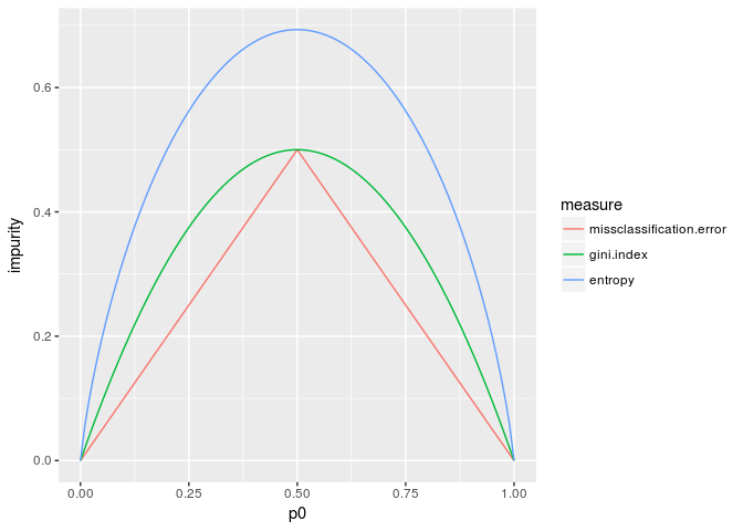
NB. Since $p_1=1-p_0$, we use only $p_0$ as an independent variable.

Missclassification error

Let us predict a color of the ball which we pick up from the box. If blue balls are more than red ones (i.e. $p_0>p_1$), then our prediction should be "blue" and the missclassification error (rate) of our prediction is $1-p_0$. If red balls are more than blue ones, then the missclassification error is given by $1-p_1$.

The missiclassification error can be described as the following symmetric formula. $$Q(p_0,p_1) = 1 - \max(p_0,p_1)$$

Gini index

The Gini index is defined to be the following formula. $$Q(p_0,p_1) = 1 - (p_0^2 + p_1^2) = 1 - \|p\|^2$$

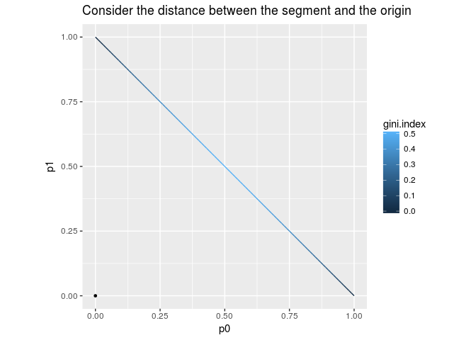
This formula is simple but we need an explanation. The space of the possible pairs $(p_0,p_1)$ form the segment connecting $(0,1)$ and $(1,0)$. The formula says: the farther the point $(p_0,p_1)$ from the origin is, the smaller the Gini index is. Therefore the middle point of the segment, i.e. $(0.5,0.5)$, maximizes the Gini index, while vertices minimize the index.

data.frame(p0=seq(from=0,to=1,by=0.01)) %>%
  mutate(p1=1-p0,
         gini.index=1-(p0^2+p1^2)) %>%
  ggplot(aes(p0,p1,color=gini.index)) + geom_line() + coord_fixed(ratio=1) +
  geom_point(data=data.frame(p0=0,p1=0),size=1,color="black") + 
  labs(title="Consider the distance between the segment and the origin")

Entropy

An entropy is defined as the expected value of an information content. Given an event $A$ with $\mathbb P(A)>0$, we define the information content of $A$ by $$I(A) := \log \left(\frac{1}{\mathbb P(A)}\right) = - \log \mathbb P (A)$$ If $\mathbb P(A) = 0$, then we set $I(A)=0$. The reason for the formula is:

• A less likely event has more information. ("snowy" has more information than "cloudy".)
• But the event which never happens has no information.
• If two independent events $A$ and $B$ happen at the same time, its information content should be some of their information contents: $I(A \cap B) = I(A) + I(B)$.

NB: We are using the natural logarithm $\log$ rather than $\log_2$.

Now the entropy is defined by $$H(p_0,p_1) = p_0I(\mathrm{blue}) + p_1 I(\mathrm{red}) = - \sum_i p_i \log(p_i) $$

Examples

Let us look at an example by using the Titanic dataset.

df <- PASWR::titanic3 %>% select(pclass,sex,fare,survived)
df <- df[complete.cases(df),]
df %>% mutate(survived=as.factor(survived)) %>%
  ggplot(aes(fare,pclass,color=survived)) + geom_point(alpha=0.4) +
  facet_grid(sex~.)

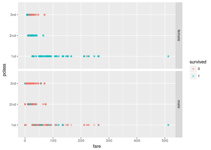
Using a pair of sex and pclass, we can divide the data into 6 buckets. The impurity measures for the buckets can be computed as follows.

df.impurity <- df %>% 
  group_by(sex,pclass) %>% 
  summarise(r.died=1-mean(survived),  ## proportion of red balls (p_0)
            r.survived=mean(survived) ## proportion of blue ones (p_1)
            ) %>%
  mutate(missclassification.error=1-pmax(r.survived,r.died), ## pmax = pairwise max
        gini.index=1-(r.died^2+r.survived^2),
        entropy=nat(r.died)+nat(r.survived)) ## nat() is defined above

The result is following.

     sex pclass     r.died r.survived missclassification.error gini.index   entropy
  <fctr> <fctr>      <dbl>      <dbl>                    <dbl>      <dbl>     <dbl>
1 female    1st 0.03472222  0.9652778               0.03472222 0.06703318 0.1507920
2 female    2nd 0.11320755  0.8867925               0.11320755 0.20078320 0.3531694
3 female    3rd 0.50925926  0.4907407               0.49074074 0.49982853 0.6929757
4   male    1st 0.65921788  0.3407821               0.34078212 0.44929934 0.6415529
5   male    2nd 0.85380117  0.1461988               0.14619883 0.24964946 0.4160585
6   male    3rd 0.84756098  0.1524390               0.15243902 0.25840274 0.4269166

Automatic segmentation, revisited

In the last entry we looked at an automatic segmentation by using Titanic dataset: fare=20 was a very good threshold to divide the data into two sets, but we could not find the threshold by using a decision tree.

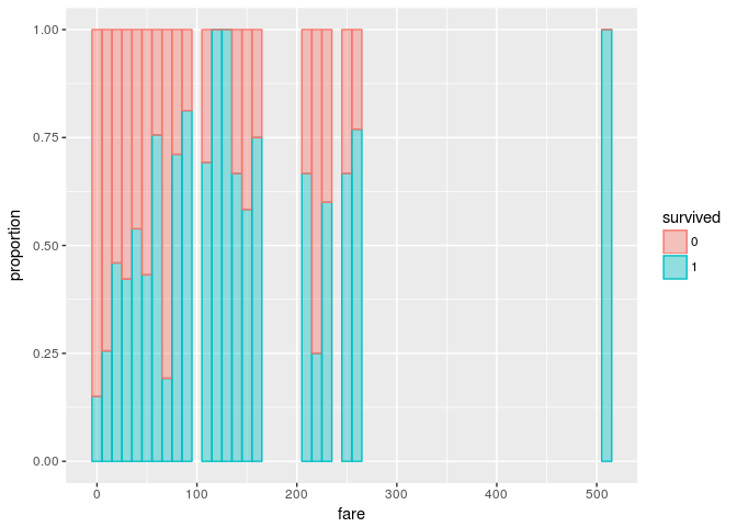
The following bar graph shows proportions of died/survived samples with respect to fare.

df %>%
  mutate(survived=as.factor(survived)) %>%
  ggplot(aes(fare,color=survived,fill=survived)) +
    geom_histogram(binwidth=10, position="fill", alpha=0.4) + 
    labs(y="proportion")

The task was to find a good threshold/segmentation for the variable "fare". If we split the fare with one threshold, we obtain two bucktets. Since for each bucket we have an impurity measure, we compute the sum of the impurity measures by threshold.

compute.impurity <- function(df,threshold) {
  df.tmp <- df %>% 
    mutate(bucket=ifelse(fare<=threshold,"A","B")) %>%
    group_by(bucket) %>%
    summarise(r.survived=mean(survived),
              r.died=1-mean(survived)) %>%
    mutate(missclassification.error=1-pmax(r.survived,r.died),
           gini.index=1-(r.died^2+r.survived^2),
           entropy=nat(r.died)+nat(r.survived)) %>%
    summarise(missclassification.error=sum(missclassification.error),
              gini.index=sum(gini.index),
              entropy=sum(entropy)*log(2)) %>%
    mutate(fare=threshold)
  return(df.tmp)
}

threshold <- sort(unique(df$fare))
threshold <- (threshold[-1] + threshold[-length(threshold)])/2

df.impurity <- lapply(threshold,function(t) compute.impurity(df,t)) %>%
  data.table::rbindlist()

df.impurity <- df.impurity %>% 
  melt(id.var="fare", 
       measure.vars=c("missclassification.error","gini.index","entropy"),
       value.name="impurity", variable.name="measure")

ggplot(df.impurity, aes(fare,impurity,color=measure)) + 
  geom_line() + 
  geom_vline(xintercept=c(20,52), size=0.1, linetype="dashed")

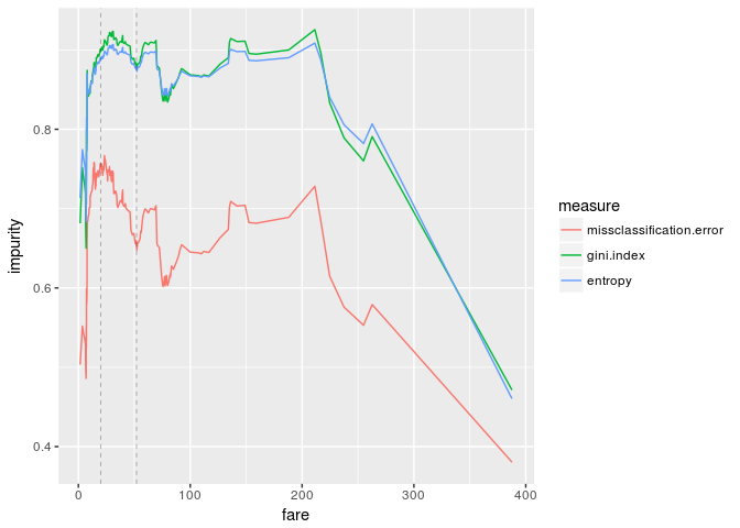
The first vertical dashed line is the "best" impurity measure (fare=20) and the second one is the threshold which we obtained by training a decision tree (fare=52). The above graphs are quite different from the results we got last time.

This is because we just added the impurity measures, or equivalently we ignored the size of the buckets. Therefore we take a product of the impurity and the proportion of the bucket and sum them.

compute.weighted.impurity <- function(df,threshold) {
  df.tmp <- df %>% 
    mutate(bucket=ifelse(fare<=threshold,"A","B")) %>%
    group_by(bucket) %>%
    summarise(r.survived=mean(survived),
              r.died=1-mean(survived),
              size=n()) %>%
    mutate(missclassification.error=1-pmax(r.survived,r.died),
           gini.index=1-(r.died^2+r.survived^2),
           entropy=nat(r.died)+nat(r.survived),
           proportion=size/nrow(df)) %>%
    summarise(missclassification.error=sum(proportion*missclassification.error),
              gini.index=sum(proportion*gini.index),
              entropy=sum(proportion*entropy)*log(2)) %>%
    mutate(fare=threshold)
  return(df.tmp)
}

df.wi <- lapply(threshold,function(t) compute.weighted.impurity(df,t)) %>%
  data.table::rbindlist()

df.wi <- df.wi %>% 
  melt(id.var="fare", 
       measure.vars=c("missclassification.error","gini.index","entropy"),
       value.name="impurity", variable.name="measure")

ggplot(df.wi, aes(fare,impurity,color=measure)) + 
  geom_line() + 
  geom_vline(xintercept=c(20,52), size=0.1, linetype="dashed")

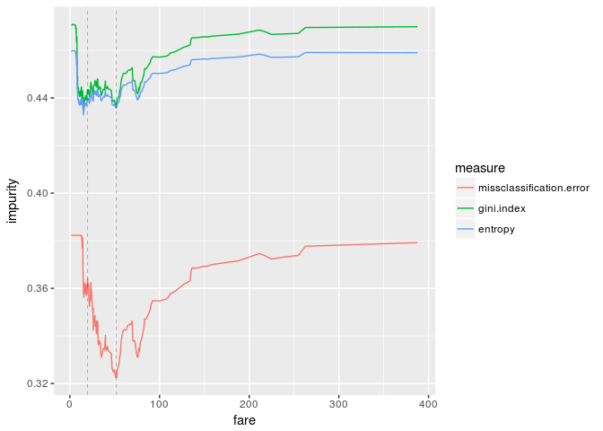
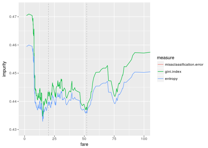
The graphs look great. If we enlarge the graphs, the threshold "fare=20" is pretty good, while our threshold is clearly good from the viewpoint of impurity measures.

ggplot(df.wi, aes(fare,impurity,color=measure)) + 
  geom_line() + 
  geom_vline(xintercept=c(20,52), size=0.1, linetype="dashed") + 
  coord_cartesian(xlim=c(0,100), ylim=c(0.43,0.473))