• Using python 3.4.5 (cf. What’s New In Python 3.0)
• scipy==0.18.0, numpy==1.9.0, matplotlib==1.5.2, sklearn==0.18.1, seaborn==0.7.1, pandas==0.18.1
• $ pip3 install --user [package] install packages under ~/.local
• install jupyter to use ipython notebook
• Spell checking in Jupyter notebooks, Emacs keybindings for Jupyter notebook

Disclaimer

• At your own risk.
• This is NOT a complete list of options. See manual for it.

General Resources

• Python 3.4.3 documentation
• Scipy Lecture Notes
• NumPy Reference
• Introduction to machine learning with scikit-learn

Template

#!/usr/bin/python3 -tt

import numpy as np
import scipy.stats as stats
import pandas as pd
import matplotlib.pyplot as plt
import seaborn as sns

# The following lines are only for Jupyter
%matplotlib inline 
from pylab import rcParams
rcParams['figure.figsize'] = 10, 5 ## width, height (inches)

Python Basics

Set Types

A constructor set() takes an iterable object. Manual.

A = set(range(3,7)) # {3, 4, 5, 6}

• Propositions: a in A, a not in A, A.issubset(B), A.issuperset(B)
• Methods for tweak: add(x), discard(x)
• Binary operations: A.intersection(B), A.union(B), A.difference(B)

Built-in modules

• itertools: product(), permutations(), combinations(), combinations_with_replacement()
• collections: Counter(), defaultdict()

Datetime

A datetime object represents a date and a time. Manual.

from datetime import datetime
from pytz import timezone

now_de = datetime.now(timezone('Europe/Berlin'))   # datetime.datetime object
now_jp = now_de.astimezone(timezone('Asia/Tokyo')) # in a different TZ

Use datetime.strptime() to convert a string into a datetime object.

datetime.strptime('2009/3/25 19:30:58', '%Y/%m/%d %H:%M:%S')

It is more practical to use pandas.to_datetime() because it automatically guesses the format. Manual.

pd.to_datetime('2009/3/25 19:30:58') # no need to give the format

The output is a pandas.tslib.Timestamp object, but we can regard it as a datetime object.

• .month, .day : return month and day, respectively.

To create a series of dates, pd.date_range is useful

pd.date_range('20160101', periods=2, freq='D')
# DatetimeIndex(['2016-01-01', '2016-01-02'], dtype='datetime64[ns]', freq='D')

Methods for a datetime object

• date() : converts a datetime object into a date object
• weekday() : gives the weekday in a number: 0 (mon) &ndash 6 (sun)
• isoformat(sep=' ') : ISO 8601 format (for SQL)

A difference of times gives a timedelta object. The .days attribute gives the time difference in days.

Files I/O

fo = open('test.txt','r') # creates a file object (for reading)
for line in fo:           # reads the file line by line
    line = line.rstrip()  # removes white spaces
    ''' ... '''
fo.close                  # close the file object

If we use a with statement, we do not need to close the file object.

with open("test.txt") as fo:
    for line in fo:
        line = line.rstrip()
        ''' ... '''

• Manual: open(), rstrip(), file object, tutorial
• fo.write("string") writes a string without "\n" in the writing mode.

JSON

• Manual
• data = json.loads(json_string)
• json_string = json.dumps(data)

Use json.load(file_obj) (not loads()) to read a JSON file.

import json
json_fo = open("sample.json",'r') # the file object of the JSON file
data = json.load(json_fo)         # read the file as a variable
json_fo.close()

Use json.dump(data,file_obj) (not dumps()) to create a JSON file.

jfo = open('write.json','w')
json.dump(data,jfo)          # store the variable "data" as a json file
jfo.close()

SQLite3

Reads a sqlite3 database and execute something row by row. Manual, Tutorial.

import sqlite3
conn = sqlite3.connect('Auto.sqlite') # a connection object
#conn.row_factory = sqlite3.Row       # for a dictionary cursor (*)
cur = conn.cursor()                   # a cursor object
cur.execute('SELECT * FROM Auto')
while True:
    ''' execute something row by row '''
    row_tuple = cur.fetchone()  # a row as a tuple (not a list!)
        if row == None:         # do not forget it
        break
    ''' do something '''
conn.close()

• cur.fetchone() returns a tuple of a row instead of a list. Use list() to convert a tuple into a list.
• cur.fetchall() returns a list of tuples of all rows.
• Using the line (*), we can create a dictionary cursor. After that cur.fetchone() returns a sqlite Row object and cur.fetchall() returns a list of Row objects. A Row object behaves like a dictionary.

A placeholder works as follows:

conn = sqlite3.connect('Auto.sqlite') # a connection object
cur = conn.cursor()                   # a cursor object
cur.execute('UPDATE Auto SET name=? WHERE cylinders=?', ('something',4))
conn.commit()
conn.close()

• A placeholder prevents an SQL injection.
• If a placeholder is only one ?, then we have to use (something,) for a tuple.
• cur.executemany() accepts a tuple of tuples instead of a tuple.

Other Databases

• MySQL: mysqlclient, other possibility.
• MongoDB: PyMongo
• Hadoop Streaming: mrjob
• Spark: PySpark, MLlib

Regular Expression

Manual, Tutorial

import re

re.sub() corresponds s/regexp/alternative/g in Perl. Manual.

re.sub('\d\d','---',"abc12def25g")                             # 'abc---def---g'
re.sub('\d\d',lambda x: str(int(x.group(0))**2),"abc12def25g") # 'abc144def625g'

re.search() corresponds /regexp/ in Perl and returns a match object.

match_obj = re.search('(\d\d).*(\d\d)','abc12de25')
match_obj.groups() # gives a tuple ('12', '25')

To get each matched string, use group(1), group(2), ... (Do not forget the parentheses.)

Use the re.I flag for the case-insensitive match.

match_obj = re.search('AB','abc12de25', re.I) # match

re.findall()

re.findall() gives the list of matched strings:

re.findall('\d\d','abc12de25') # ['12', '25'] # (global match)

Mathematics and Statistics (numpy)

NumPy Reference. This section is basically part of An introduction to Numpy and Scipy.

Creating array objects

A (multi-dimensional) matrix can be represented as an array object (a.k.a. ndarray). The easiest ways to create one is to give a list to the np.array() function. Its size can be changed by reshape() method.

import numpy as np
np.array([[1,2,3],[4,5,6]])         # 2x3 matrix
# [[1 2 3]
#  [4 5 6]]
np.array(range(1,7)).reshape((2,3)) # the same matrix as above
np.arange(1,7).reshape((2,3))       # this is also the same

To make a copy of an array object, use the copy() method.

• np.arange(4) : same as np.array(range(4)).
• np.zeros((2,3)) : the 2x3 matrix consisting only of 0
• np.ones((2,3)) : the 2x3 matrix consisting only of 1
• np.identity(2) : the 2x2 identity matrix
• np.diag([2,3]) : $\mathrm{diag}(2,3)$
• np.linspace(0,1,num=100) : divides the closed interval $[0,1]$ with 100 points

Manipulation and slices

Use the shape property to find the size of an array object.

a = np.zeros((3,4))
a.shape             # tuple (3,4)
a.shape[0]          # 3
np.arange(2).shape  # (2,) 

The last array is a 1-dimentional array. Use np.newaxis to make it a row/column vector (or the reshape() method):

a = np.arange(3) # 1-dim array   (3,)
a[:,np.newaxis]  # column vector (3,1)
a[np.newaxis,:]  # row vector    (1,3)

We can slice part of an array as follows. (We should be careful about dimension.)

a = np.array([[1,2,3],[4,5,6]])
a[0,0]   # 1
a[1,:]   # the 2nd row [4,5,6]  (1-dim array!)
a[:,2]   # the 3rd column [3,6] (1-dim array!)
a[:,0:2] # the following 2x2 matrix
# [[1, 2]
#  [4, 5]]
a[:,0:2] = np.identity(2) # A slice accepts a substitution 
# [[1, 0, 3]
#  [0, 1, 6]]

The np.concatenate() function concatenates two arrays

a = np.arange(2)[np.newaxis,:]       # 1x2 matrix (row vector)
b = np.array([99,100])[np.newaxis,:] # 1x2 matrix (row vector)
np.concatenate((a,b),axis=0)         # rbind()
# [[  0   1]                         # (1+1)x2 matrix
#  [ 99 100]]
np.concatenate((a,b),axis=1)         # cbind()
# [[  0   1  99 100] ]               # 1x(2+2) matrix

Linear algebra

np.pi and np.e give the mathematical constants. A lot of mathematical functions such as np.abs(), np.sqrt(), np.log() are available. The np.sign() function returns the sign of an element as 1, 0 or -1.

np.sign(np.arange(-2,3)) # [-1, -1,  0,  1,  1]

The coordinate-wise binary operations: +, -, *, /, % (reminder). If the shapes of two matrices do not agree, then smaller one will be broadcasted. For example,

a = np.arange(1,7).reshape((2,3)) # 2x3 matrix
# [[1 2 3]
#  [4 5 6]]
c = (np.arange(3)-1)[np.newaxis]  # 1x3 matrix
# [[-1,  0,  1] ]
a+c
# [[0, 2, 4]      # '+c' is applied to all rows
#  [3, 5, 7]]
d = np.array([10,-10]).reshape((2,1)) # 2x1 matrix
# [[ 10]
#  [-10]]
a*d
# [[ 10  20  30]  # '*d' is applied to all columns
#  [-60 -50 -40]]

If the larger matrix is square, then it is ambiguous how the array will be broadcasted. So it is a best practice to specify its shape by np.newaxis or reshape().

A multiplication of two matrices can be calculated by np.dot(). As its name suggests, it computes the dot product of two vectors (1-dim arrays).

np.dot(np.arange(3),np.array([0,3,10])) # 23

• np.cross(u,v) : the cross product $\vec u \times \vec v$ of two vectors
• np.outer(np.arange(1,10),np.arange(1,10)) : multiplication table
• X.tranpose() : $X^T$.

numpy.linalg

numpy.linalg contains lots of functions for linear algebra.

• np.linalg.matrix_power(A,8) : $A^8$
• np.linalg.inv(A) : $A^{-1}$
• np.trace(A) : $\mathrm{trace}(A)$. This is NOT in linalg.
• np.linalg.det(A) : $\det A$
• np.linalg.matrix_rank(A) : $\mathrm{rank}(A)$. This makes use of SVD.
• np.linalg.norm(A) : Frobenius norm $\sqrt{\mathrm{trace}(A^TA)}$. More norms are available.

np.linalg.eig() computes eigenvalues and eigenvectors.

X = np.array([1,2,3,2,4,5,3,5,6]).reshape((3,3))
# [[1, 2, 3]
#  [2, 4, 5]
#  [3, 5, 6]]
evals, evecs = np.linalg.eig(X)
evals # eivenvalues (1-dim array)
# [ 11.34481428,  -0.51572947,   0.17091519]
evecs # evecs[:,i] is an evals[i]-eigenvector.
# [[-0.32798528, -0.73697623,  0.59100905]
#  [-0.59100905, -0.32798528, -0.73697623]
#  [-0.73697623,  0.59100905,  0.32798528]]
np.dot(vecs, np.dot(np.diag(vals), np.linalg.inv(vecs))) # = X

The np.linalg.svd() function computes the singular value decomposition. Manual.

X = np.arange(15).reshape((3,5))
# [[ 0,  1,  2,  3,  4]
#  [ 5,  6,  7,  8,  9]
#  [10, 11, 12, 13, 14]]
U, s, Vt = np.linalg.svd(X)
S = np.diag(s)                       # makes s a diagonal matrix
np.dot(U, np.dot(S, Vt[0:len(s),:])) # very close to X

The actual size of U and Vt depend on the shape of X, so let us assume that $X$ is an $n \times p$ matrix with $n \leq p$. Then the SVD of $X$ is a decomposition $X=USV^T$ such that

• $S$ : the root of the $n \times n$ diagonal matrix of eigenvalues of the symmetric matrix $XX^T$.
• $U \in O(n)$ : the matrix the eigenvectors $XX^T$.
• $V$ : a $p \times n$ matrix whose columns are principal components of $X$. This is orthonormal in the sense that $V^TV = 1$.

The matrix Vt which np.linalg.sdv() gives $\tilde V^T$, where $\tilde V \in O(p)$ is an orthogonal extension of $V$. (Namely the orthonormal basis of $\ker(X)$ are added.)

Aggregation functions

Aggregation methods: sum(), prod(), mean(), var(), std(), max(), min(). Add the axis option to apply one of the methods along an axis.

X = np.array([-7,2,3,5,1,7,-4,8]).reshape((2,4))
# [[-7,  2,  3,  5]
#  [ 1,  7, -4,  8]]
X.sum(axis=0)        # sum() along the first axis
# [-6,  9, -1, 13]   # 1-dim array
X.max(axis=1)        # max() along the second axis
# [5, 8]             # 1-dim array

Note that np.median() is a function.

Let $x^1$, ... , $x^n$ be row vectors of a matrix $X$. np.cov() computes the covariance of these vectors (i.e. the covariance matrix).

np.cov(X) # X is the 2x4 matrix as above.
# [[ 28.25      ,   8.66666667]
#  [  8.66666667,  31.33333333]]

The (i,j)-component of np.cov(X) is $\frac{1}{n-1}\langle x^i_c, x^j_c\rangle$, where $x^i_c$ is the centred vector of $x^i$.

The correlations of rows can be computed by the np.corrcoef() function.

np.corrcoef(X) # X is the 2x4 matrix as above.
# [[ 1.        ,  0.29129939]
#  [ 0.29129939,  1.        ]]

Its $(i,j)$-component is equal to $\frac{1}{n-1}\langle x^i_n, x^j_n\rangle$, where $x^i_n$ is the normalised vector of $x^i_c$.

Use seaborn to draw a heat map of the correlation matrix: sns.heatmap(np.corrcoef(X)).

Random sampling (numpy.random)

• Manual.
• np.random.seed(2016) sets a random seed
• np.random.choice(array, size=None, replace=True) returns random samples from the given array.

Statistical functions (scipy.stats)

scipy.stats consists of many functions for statistics.

Well-known distributions

Normal distribution

The PDF of $\mathcal N(\mu,\sigma)$ is given by $p(x) = \dfrac{1}{\sqrt{2\pi\sigma^2}}\exp\left(-\dfrac{(x-\mu)^2}{2\sigma^2}\right)$.

• stats.norm.rvs(loc=0,scale=1,size=50) : draws random samples
• stats.norm.pdf(x,loc=0,scale=1) : probability density function
• stats.norm.cdf(x,loc=0,scale=1) : cumulative density function
• stats.norm.ppf(x,loc=0,scale=1) : percent point function (inverse of CDF)
• A multivariate normal distribution $\mathcal N(\mu,\Sigma)$ is also available.

Replacing norm with other term, we can use other continuous distribution in a similar way.

Uniform distribution

The PDF of $\mathsf U(a,b)$ is given by $p(x) = \dfrac{1_{[a,b]}(x)}{b-a}$.

• stats.uniform.rvs(loc=0,scale=1,size=50) : draws random samples
• stats.uniform.pdf(x,loc=0,scale=1) : PDF
• loc means $a$ and scale means $b-a$.

Exponential distribution

The PDF of $\mathsf{Exp}(\lambda)$ is given by $p(x) = \lambda e^{-\lambda x}1_{[0,\infty)}$.

• stats.expon.rvs(scale=1, size=50) : draws random samples
• stats.expon.pdf(x,scale=1) : PDF
• scale means $1/\lambda$, which equals to the standard deviation.

Binomial distribution

The PMF of $\mathsf{Bin}(n,p)$ is given by $\mathbb P(X=x) = \begin{pmatrix} n \\ x\end{pmatrix} p^x(1-p)^{n-x}$ for $x = 0, \cdots, n$.

• stats.binom.rvs(n,p,size=50) : draws random samples
• stats.binom.pmf(x,n,p) : PMF (not PDF)
• stats.binom.cdf(x,n,p) : CDF
• stats.binom.ppf(x,n,p) : percent point function (the "inverse" of CDF)

Replacing binom with other term, we can use other discrete distribution in a similar way.

Possion distribution

The PMF of $\mathsf{Poisson}(\mu)$ is given by $\mathbb P(X=k) = \dfrac{\mu^k}{k!}e^{-\mu}$ for $k = 0, 1, 2, \cdots$.

• stats.poisson.rvs(mu, size=1)
• stats.poisson.pmf(k, mu) : PMF

Welch's t-test

• Assumptions: two random variables are normally distributed.
• Null Hypothesis: two random variables has the same expected value.

scipy.stats.ttest_ind() computes the p-value. Manual.

a = st.norm.rvs(loc=11,scale=5,size=200)   # population A 
b = st.norm.rvs(loc=10,scale=5.2,size=200) # population B
tstat, pval = st.ttest_ind(a, b, equal_var=False)

Fisher's exact test

• Assumptions: two random variables are Bernoulli distributed.
• Null Hypothesis: two random variables has the same expected value.

scipy.stats.fisher_exact() computes the p-value. Manual. But we have to calculate a crosstab in advance.

a = st.bernoulli.rvs(0.03, size=1200)  ## population A
b = st.bernoulli.rvs(0.035, size=1000) ## population B
pos = np.array([a.sum(), b.sum()])     ## 1st row
neg = np.array([1200, 1000]) - pos     ## 2nd row
ctab = np.array([neg,pos])             ## 2x2 table
oddsratio, pval = st.stats.fisher_exact(ctab)

A chi-squared test for goodness of fit

• Assumptions: two random variables are multinomial distributed.
• Null Hypothesis: two random variables are independent.

scipy.stats.chi2_contingency() computes the p-value. Manual. We have to compute the crosstab in advance. (pandas.crosstab() is convenient for the computation.)

a = ['abc'[x] for x in st.randint.rvs(0,3,size=300)]    ## variable 1 
b = ['yn'[x] for x in st.bernoulli.rvs(0.35, size=300)] ## variable 2
ctab = pd.crosstab(pd.Series(a, name='A'), pd.Series(b, name='B'))
chi2, pval, dof, expected = st.chi2_contingency(ctab)

Other useful modules

• scipy.special (Manual). lbeta, etc.
• scipy.optimize (Manual). for gradient descent, etc. Note that the argument of the objective function must be an array.

DataFrame (pandas)

• pandas : the official website
• Intro to pandas data structures, An introduction to Pandas : tutorials

Note that we need to use print() to print the actual data in the following codes (not on the IPython).

Series

A Series is like list with keys (index). We can create one from an usual list as follows.

x = pd.Series(['a','b','c'], index=range(3))
x
# 0    a
# 1    b
# 2    c
# dtype: object

An object of Series behaves like a list in R.

x == 'a'
# 0     True
# 1    False
# 2    False
# dtype: bool
x[x=='a']
0    a
dtype: object

Examples of methods mean(), unique(), nunique(), value_counts(), etc.

np.random.seed(0)
x = pd.Series(np.random.randint(0,4,size=10))
x.unique()  ## array([0, 3, 1])
x.nunique() ## len(x.unique()) i.e. 3 
x.value_counts()
# 3    6
# 1    2
# 0    2
# dtype: int64

DataFrame

Something like a data frame in R.

data = {
    'col1' : range(1,9),
    'col2' : [x**2 for x in range(1,9)],
    'col3' : [np.exp(x) for x in range(1,9)],
}
df = pd.DataFrame(data,columns=['col1','col2','col3']) # dict -> data frame

CSV

The method read_csv() is used to read a CSV file

df = pd.read_csv("file",sep=',')

• file : a file location or a URL of the CSV
• index_col=None : the column number of indexes
• header=None, names=cols : If the file contains no header, we give names to the columns with names (not columns)
• na_values='?' : specified string is recognised as a NaN
• decimal='.' : decimal point
• thousands=None : thousands separator
• dtype={'age':np.int64} : specified the type of a column
• converters={'date':pd.to_datetime} : apply a function to values in a column

To save an object of DataFrame, use df.to_csv("output.csv",index=False).

SQLite3

See the documentation for more details..

from pandas.io import sql
import sqlite3

conn = sqlite3.connect('db.sqlite')
query = "SELECT rowid,* FROM Table;"
df = sql.read_sql(query, con=conn)

See the data frame

url = "http://www-bcf.usc.edu/~gareth/ISL/Auto.csv"
df = pd.read_csv(url, na_values='?')

• df.shape : tuple of the numbers of rows and columns
• df.info() : check the types of columns (find columns in "object")

df.describe() is something like summary(df) in R. (Note that the column of "object" is ignored):

              mpg   cylinders  displacement       weight  acceleration  \
count  397.000000  397.000000    397.000000   397.000000    397.000000   
mean    23.515869    5.458438    193.532746  2970.261965     15.555668   
std      7.825804    1.701577    104.379583   847.904119      2.749995   
min      9.000000    3.000000     68.000000  1613.000000      8.000000   
25%     17.500000    4.000000    104.000000  2223.000000     13.800000   
50%     23.000000    4.000000    146.000000  2800.000000     15.500000   
75%     29.000000    8.000000    262.000000  3609.000000     17.100000   
max     46.600000    8.000000    455.000000  5140.000000     24.800000   

             year      origin  
count  397.000000  397.000000  
mean    75.994962    1.574307  
std      3.690005    0.802549  
min     70.000000    1.000000  
25%     73.000000    1.000000  
50%     76.000000    1.000000  
75%     79.000000    2.000000  
max     82.000000    3.000000

Rows and columns

The "index" of rows (resp. columns) start from 0.

• df.columns : list of the column names
• df.index : list of the row indexes
• df.values : convert df into an ndarray object of numpy

The column named weight can be access by df['weight'] or df.weight.

0      3504
1      3693
       ... 
395    2625
396    2720
Name: weight, dtype: int64

If "values" is used as a label of a column, df.values gives the result of the method values. Because many methods are defined on a data frame, we should NOT use df.col_name to get a column series.

We may change a label of a column by rename method.

df.rename(columns={'horsepower':'pow'},inplace=True) ## 'pow' is also a method...

Or we can assign a complete list of labels:

df.columns = ['mpg','cyl','disp','pow','weight','acc','year','origin','name']
df.index = ["r%s" % i for i in range(1,df.shape[0]+1)] ### We start with "r1"!

df.set_index('column_name',inplace=True) makes to make a column the row indexes.

While df['cyl'] gives the Series of the column "cyl", df.ix["r100"] gives the Series of the row "r100".

mpg               18
cyl                6
disp             232
pow              100
weight          2945
acc               16
year              73
origin             1
name      amc hornet
Name: r100, dtype: object

Then df.ix["r100","weight"] gives the 2945.

df.ix accepts the notation :. For example df.ix["r100":"r103","cyl":"year"] gives

      cyl  disp  pow  weight   acc  year
r100    6   232  100    2945  16.0    73
r101    6   250   88    3021  16.5    73
r102    6   198   95    2904  16.0    73
r103    4    97   46    1950  21.0    73

To specify all columns (or rows) we may leave only :. For example df.ix[99:102,:] gives

      mpg  cyl  disp  pow  weight   acc  year  origin                     name
r100   18    6   232  100    2945  16.0    73       1               amc hornet
r101   18    6   250   88    3021  16.5    73       1            ford maverick
r102   23    6   198   95    2904  16.0    73       1          plymouth duster

Note that df.index[99] is "r100" and df.index[102] is "r103". (We have assigned r1 to df.index[0].) Namely the behaviour of : depends which we use to specify rows (or columns): labels or coordinates.

Remark. There are other ways to get values by using coordinates or labels.

The function pd.crosstab produces a contingency table.

pd.crosstab(df['cyl'],df['year'])
# year  70  71  72  73  74  75  76  77  78  79  80  81  82
# cyl                                                     
# 3      0   0   1   1   0   0   0   1   0   0   1   0   0
# 4      7  13  14  11  15  12  15  14  17  12  25  21  27
# 5      0   0   0   0   0   0   0   0   1   1   1   0   0
# 6      4   8   0   8   7  12  10   5  12   6   2   7   3
# 8     18   7  13  20   5   6   9   8   6  10   0   1   0

Conversion of a data type

Convert an "object" to a "float".

df['pow'].dtype                                      # dtype: object
df['pow'] = pd.to_numeric(df['pow'],errors='coerce') # dtype: float64

Convert a date string (object) to a datetime object.

s = pd.Series(['12/1/2012', '30/01/2012']) # dtype: object
s = pd.to_datetime(s, format='%d/%m/%Y')   # dtype: datetime[64]

to_datetime() can guess the format of the date automatically. So we leave out the format option, but the process will be faster if the format is given.

Convert a column to a categorical data.

df['origin'].unique()                # [1 3 2] # dtype: int64
df['origin'] = df['origin'].astype('category') # dtype: category
df['name'].dtype                               # dtype: object
df['name'] = df['name'].astype('category')     # dtype: category

The following code makes the categories more meaningful.

df['origin'].cat.categories = ['usa','europe','japan']

Concatenate dataframes

• pd.concat([df,dg]) : equivalent to rbind(df,dg) in R.
• pd.concat([df,dg],axis=1) : equivalent to cbind(df,dg) in R.

Merge

data1 = {'rowid' : range(1,4), 'col1' : range(10,13),}
df = pd.DataFrame(data1,columns=['rowid','col1'])
data2 = {'rowid' : range(2,5), 'col2' : ['a','b','c'],}
dg = pd.DataFrame(data2,columns=['rowid','col2'])

pd.merge(df,dg,on='rowid',how='inner') merge two dataframes for only common rowids.

   rowid  col1 col2
0      2    11    a
1      3    12    b

how='left' (resp. how='right') option keeps all rows of the first (resp. second) dataframe.

   rowid  col1 col2
0      1    10  NaN
1      2    11    a
2      3    12    b

how='outer' option keeps all rows of the both dataframes.

Applying a function to a column/row

To apply a function to each column, use apply method.

dg = df.ix[:,'mpg':'acc']  # consists only of numerical columns.
dg.apply(np.median,axis=0) # applying an aggregate function
# mpg         23.0
# cyl          4.0
# disp       146.0
# pow         95.0
# weight    2800.0
# acc         15.5
# dtype: float64
dg.apply(lambda x: np.log(x+1)).head(3) # applying a component-wise function
#          mpg       cyl      disp       pow    weight       acc
# r1  2.944439  2.197225  5.730100  4.875197  8.161946  2.564949
# r2  2.772589  2.197225  5.860786  5.111988  8.214465  2.525729
# r3  2.944439  2.197225  5.765191  5.017280  8.142354  2.484907

We may also use apply method for a series, when we want to apply a component-wise function.

df['disp'].apply(lambda y: np.log(y+1)).head(3)
# r1    5.730100
# r2    5.860786
# r3    5.765191
# Name: disp, dtype: float64

If we want to apply an aggregate function (of numpy) to a series, use it directly.

np.median(df['disp']) # 146.0

To apply a function to each row, use axis=1 option.

Missing data

Working with missing data.

• pd.isnull(df) gives a boolean data frame giving "True" where "NaN" was there.
• df.dropna(how='any') gives only rows without "NaN".
• df.fillna(value=0) fills "0" at missing points.

To count the number of NA by column:

from collections import Counter
pd.isnull(df).apply(lambda x: Counter(x)[True])
# mpg       0
# cyl       0
# disp      0
# pow       5
# weight    0
# acc       0
# year      0
# origin    0
# name      0
# dtype: int64

To see the rows with a missing value, we make a boolean series as follows.

from collections import Counter
row_with_na = pd.isnull(df).apply(lambda x: Counter(x)[True]>0,axis=1)
df[row_with_na]
#        mpg  cyl  disp  pow  weight   acc  year origin                  name
# r33   25.0    4    98  NaN    2046  19.0    71      1            ford pinto
# r127  21.0    6   200  NaN    2875  17.0    74      1         ford maverick
# r331  40.9    4    85  NaN    1835  17.3    80      2  renault lecar deluxe
# r337  23.6    4   140  NaN    2905  14.3    80      1    ford mustang cobra
# r355  34.5    4   100  NaN    2320  15.8    81      2           renault 18i

From a wide table to a long one, and back

We use the following wide data frame.

dg = df[['mpg','disp','pow','name']].head(2)
#     mpg  disp  pow                       name
# r1   18   307  130  chevrolet chevelle malibu
# r2   15   350  165          buick skylark 320

The pd.melt() method makes a wide data frame into a long one.

dg.reset_index(inplace=True) # row indexes -> a column
dg_long = pd.melt(dg,id_vars=['index'])
    index variable                      value
# 0    r1      mpg                         18
# 1    r2      mpg                         15
# 2    r1     disp                        307
# 3    r2     disp                        350
# 4    r1      pow                        130
# 5    r2      pow                        165
# 6    r1     name  chevrolet chevelle malibu
# 7    r2     name          buick skylark 320

The pivot() method makes a long data frame into a wide one.

dg_wide = dg_long.pivot(index='index',columns='variable',values='value')
# variable disp mpg                       name  pow
# index
# r1        307  18  chevrolet chevelle malibu  130
# r2        350  15          buick skylark 320  165

When the data table has duplicate rows, we should use pivot_table().

Functions corresponding to dplyr

Warning. One of the important properties of dplyr of R is: the output is always a new data frame. But I have not checked whether (most of) the following codes produce new data frame or not. If not, we might want to use the copy method.

filtering rows

If s is a boolean series, then df[s] consists of rows where "s" is True.

df[ (df['mpg'] == 18) & (df['acc'] <= 12) ] # Don't forget the round brackets!
#     mpg  cyl  disp  pow  weight  acc  year origin                       name
# r1   18    8   307  130    3504   12    70      1  chevrolet chevelle malibu
# r3   18    8   318  150    3436   11    70      1         plymouth satellite

The isin() method may be useful.

df[ df['name'].isin(['honda civic cvcc','toyota corolla 1200']) ]
#        mpg  cyl  disp  pow  weight   acc  year origin                 name
# r54   31.0    4    71   65    1773  19.0    71      3  toyota corolla 1200
# r132  32.0    4    71   65    1836  21.0    74      3  toyota corolla 1200
# r182  33.0    4    91   53    1795  17.5    75      3     honda civic cvcc
# r249  36.1    4    91   60    1800  16.4    78      3     honda civic cvcc

When using a regular expression, we should use bool function to get a boolean series.

df[ df['name'].apply(lambda x: bool(re.search('^h.*c$',x))) ]
#        mpg  cyl  disp  pow  weight   acc  year origin               name
# r150  24.0    4   120   97    2489  15.0    74      3        honda civic
# r182  33.0    4    91   53    1795  17.5    75      3   honda civic cvcc
# r199  33.0    4    91   53    1795  17.4    76      3        honda civic
# r217  31.5    4    98   68    2045  18.5    77      3  honda accord cvcc
# r249  36.1    4    91   60    1800  16.4    78      3   honda civic cvcc
# r383  38.0    4    91   67    1965  15.0    82      3        honda civic

arrange rows

df.sort_values(by="disp",ascending=True) sorts rows by values of "disp". The option ascending is "True" by default. The option by accepts a list as well.

df.sort_values(by=["disp","pow"])).head(5)
#        mpg  cyl  disp  pow  weight   acc  year origin                 name
# r118  29.0    4    68   49    1867  19.5    73      2             fiat 128
# r112  18.0    3    70   90    2124  13.5    73      3            maxda rx3
# r72   19.0    3    70   97    2330  13.5    72      3      mazda rx2 coupe
# r335  23.7    3    70  100    2420  12.5    80      3        mazda rx-7 gs
# r54   31.0    4    71   65    1773  19.0    71      3  toyota corolla 1200

select columns

If s is a list of column names, then df[s] gives a data frame consisting of columns in s.

cols = ['pow','mpg','cyl']
df[cols].head(3)
#     pow  mpg  cyl
# r1  130   18    8
# r2  165   15    8
# r3  150   18    8

Use the drop(cols, axis=1) method to remove a few columns. Manual.

mutate

Unfortunately I have not found any standard way to achieve mutate of R in Python. Because many operation such as "+" can be applied to series by coordinates,

df['new_col'] = 3*df['mpg']**2 - 4*df['pow']

adds a column "new_col" to "df". Or we may use apply(func,axis=0) to apply a function taking a series of a row.

df['new_col'] = df.apply(lambda x: 3*x['mpg']**2-4*x['pow'], axis=1)

When we need a new data frame, use df_new = df.copy() to duplicate a data frame.

Grouping

groupby('col_name') method splits a data frame by values of 'col_name' so that we can deal with them at the same time. (Manual)

df['origin'].unique()
# [1, 3, 2]
# Categories (3, int64): [1, 3, 2]
df.groupby('origin').mean()
#              mpg       cyl        disp         pow       weight        acc  \
# origin                                                                     
# 1       20.071774  6.258065  246.284274  119.048980  3363.250000  15.011694
# 2       27.891429  4.157143  109.142857   80.558824  2423.300000  16.787143
# 3       30.450633  4.101266  102.708861   79.835443  2221.227848  16.172152
# 
#              year  
# origin             
# 1       75.584677  
# 2       75.814286  
# 3       77.443038 

The method groupby accepts a list of column names as well.

Visualisation (matplotlib, seaborn)

• matplotlib, Gallery, Pyplot tutorial, User's Guide (including Beginner's Guide)
• Seaborn, API, Gallery
• Visualisation through pandas
• Python data visualizations on the Iris dataset

The following code produces a 400x400 image "graph.png".

plt.figure(figsize=(400/96,400/96),dpi=96)
''' plot something ... '''
plt.tight_layout()  # when producing a small image 
plt.savefig('graph.png',dpi=96)

Using plt.show() instead plt.savefig(), we obtain an image window. Note that need %matplotlib inline to show the image on IPython Notebook.

Simple diagrams

• A basic strategy is: use pandas or seaborn if possible.
• pandas often requires a wide table. Use pivot(columns=, values=) (with or without index option).
• Some methods raises an error if there is a missing value in a data. Use dropna(how='any') in such a case.

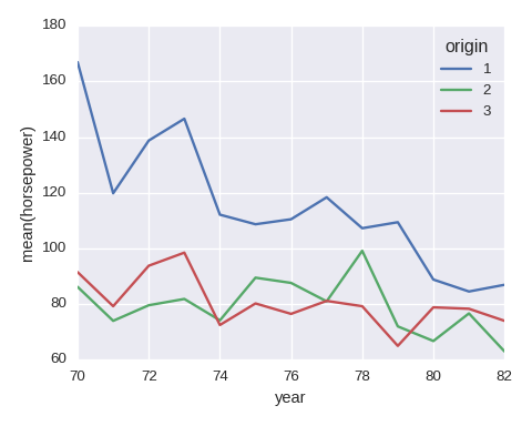
Line chart

df_tmp = df.groupby(['year','origin'])['horsepower']\
           .agg({'avg':np.mean}).reset_index()
df_tmp.pivot(index='year',columns='origin',values='avg').plot()
plt.ylabel('mean(horsepower)')

Histogram

Put stacked=True in plt.hist() if a stacked histgram is needed.

yvals = sorted(df.origin.unique())
data = [df.weight[df.origin==y].dropna(how='any') for y in yvals]
plt.hist(data,bins=20,label=yvals)
plt.xlabel('weight')
plt.ylabel('count')

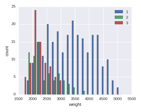
The simplest histogram can be obtained df.weight.hist().

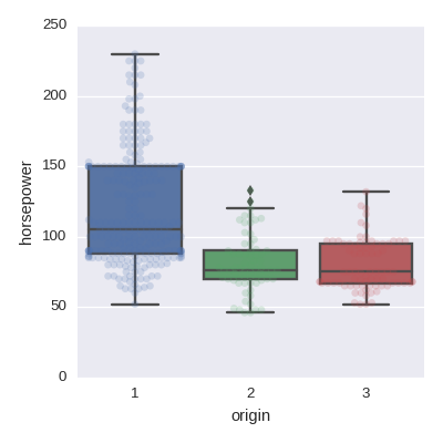
Box plot

sns.boxplot(x='origin',y='horsepower',data=df,orient='v')
sns.swarmplot(x='origin',y='horsepower',data=df,orient='v',alpha=0.2)

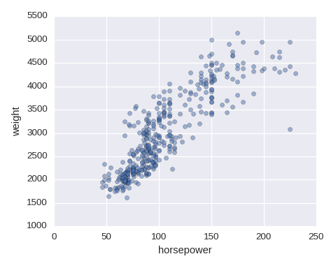
Scatter plot

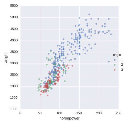
df.plot.scatter(x='horsepower',y='weight',alpha=0.5)

To add a color from a categorical variable, use FacetGrid. size=5 is for the size of the image

num1,num2 = 'horsepower', 'weight'
sns.FacetGrid(df,hue="origin",size=5)\
   .map(plt.scatter,num1,num2,alpha=0.5).add_legend()

Examples of visualisation

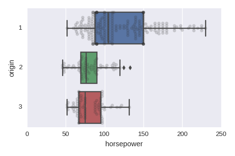
A numerical variable vs a categorical variable

sns.boxplot(x='horsepower',y='origin',data=df,orient='h')
sns.swarmplot(x='horsepower',y='origin',data=df,orient='h',color='0.2',alpha=0.2)

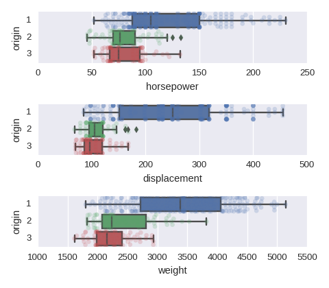
Numerical variables vs a categorical variable

To adjust the size of the image put figsize=(480/96,420/96) in plt.subplots().

cols = ['horsepower','displacement','weight']
fig, axes = plt.subplots(nrows=len(cols),ncols=1)

for col,subax in zip(cols,list(axes.flat)):
    sns.boxplot(x=col,y='origin',data=df,orient='h',ax=subax)
    sns.swarmplot(x=col,y='origin',data=df,orient='h',alpha=0.2,ax=subax)

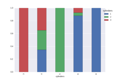
A categorical variable vs a categorical variable

The proportions of the target values in each value. (The size is not adjustable.)

cat1,cat2 = 'cylinders','origin' # cat vs cat
df_gb0 = df.groupby([cat1,cat2]).size().rename('cnt').reset_index()
df_gb1 = df_gb0.groupby(cat1)['cnt'].agg({'size':np.sum}).reset_index()
df_tmp = pd.merge(df_gb0,df_gb1,on=cat1)
df_tmp['rate'] = df_tmp['cnt']/df_tmp['size']
df_tmp = df_tmp.pivot(index=cat1,columns=cat2,values='rate').fillna(0)

df_tmp.plot.bar(stacked=True)
plt.legend(bbox_to_anchor=(1.1, 1),title=cat1)

The histogram is easy to draw.

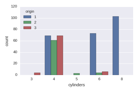
sns.countplot(x='cylinders',hue='origin',data=df)

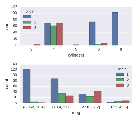
Categorical variables vs a categorical variable

df.mpg = pd.cut(df.mpg,bins=4) ## a new cat variable

cols = ['cylinders','mpg']
fig, axes = plt.subplots(nrows=len(cols),ncols=1,figsize=(480/96,420/96))
for col,subax in zip(cols,list(axes.flat)):
    sns.countplot(x=col,hue='origin',data=df,ax=subax)

A numerical variable vs a numerical variable

See the section "scatter plot" above.

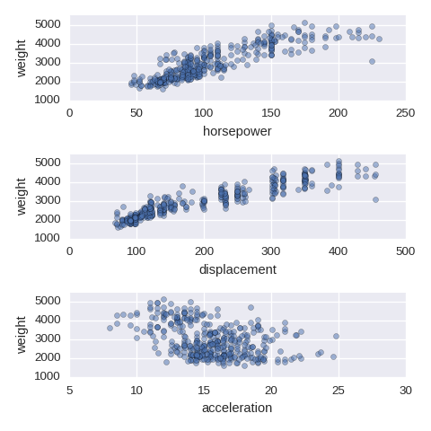
Numerical variables vs a numerical variable

If there are too many ticks on the y-axis, then use mathplotlib.ticker.MultipleLocator.

import matplotlib.ticker as ticker ## if needed

cols = ['horsepower','displacement','acceleration']
fig, axes = plt.subplots(nrows=len(cols),ncols=1,figsize=(480/96,480/96))
for col,subax in zip(cols,list(axes.flat)):
    df.plot.scatter(x=col,y='weight',alpha=0.5,ax=subax)
    subax.yaxis.set_major_locator(ticker.MultipleLocator(1000)) # if needed

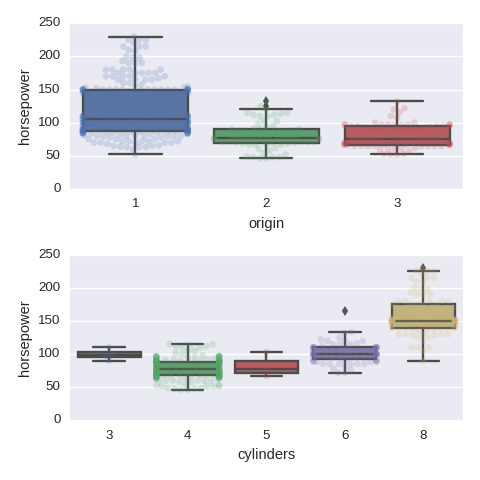
A categorical variable vs a numerical varaible

See section "Box plot" above.

Categorical variables vs a numerical varaible

cols = ['origin','cylinders']
fig, axes = plt.subplots(nrows=len(cols),ncols=1,figsize=(480/96,480/96))

for col,subax in zip(cols,list(axes.flat)):
    sns.boxplot(x=col,y='horsepower',data=df,orient='v',ax=subax)
    sns.swarmplot(x=col,y='horsepower',data=df,orient='v',alpha=0.2,ax=subax)

Pairwise relationships between numerical variables

sns.pairplot() shows pairwise relationships between (all) pairs of numerical variables.

cols = ['mpg','displacement','acceleration','origin']
df_tmp = df[cols].copy()
df_tmp.origin = df_tmp.origin.map({1:'usa',2:'eur',3:'jpn'})
sns.pairplot(df_tmp,hue='origin',size=2)

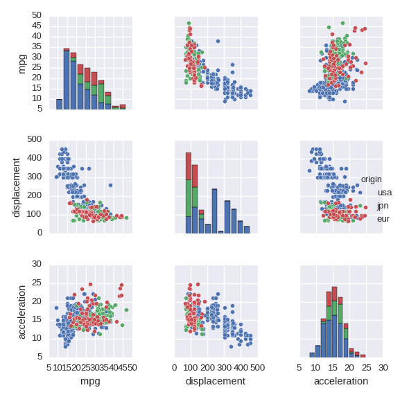
• For the hue option a categorical variable must be non numerical. Even a string of a number (such as '1') is not allowed.
• size specifies the size of the image.

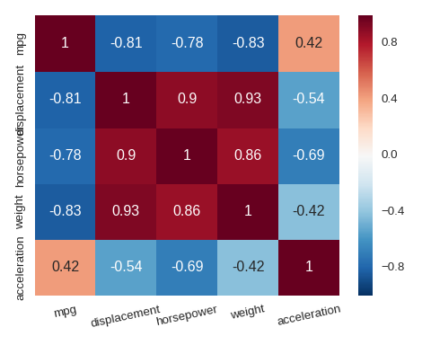
Heat map

sns.heatmap() can be used to visualise a matrix such as a correlation matrix.

cols = ['mpg','displacement','horsepower','weight','acceleration']
plt.xticks(rotation=12)
sns.heatmap(df[cols].corr(),annot=True)

Machine Learning (scikit-learn)

• scikit-learn, API reference

The feature matrix and the response vector are the NumPy arrays and stored on different variables: X and y, respectively. They are allowed to have only numerical values.

sample data

sklearn.datasets

iris = load_iris()
print(iris.DESCR) # show the description of the dataset.
X = pd.DataFrame(iris.data,columns=iris.feature_names)
y = pd.Series(iris.target,name='class')

To obtain an array of objects (rather than the numbers) for the target variable, we use iris.target_names:

[ iris.target_names[c] for c in iris.target ]

Train-Test split

from sklearn.model_selection import train_test_split
X_train,X_test,y_train,y_test = train_test_split(X,y,test_size=0.4,random_state=4)

random_state is something like seed().

Label Binalizer

We have to convert a categorical column into a pivot table. But we should use LabelBinarizer to create a table instead of pandas pivot() for consistency.

from sklearn.preprocessing import LabelBinarizer
lb = LabelBinarizer()
lb.fit(y)

pd.DataFrame(lb.transform(y), columns=lb.classes_) ## pivot table

The following function creates a function converting a categorical column (series) into a pivot table.

def pivot(vec,vals=None):
    if vals is None:
        vals = vec.unique()
    lb = LabelBinarizer().fit(vec)

    def create_df(series):
        pivot_df = pd.DataFrame(lb.transform(series),columns=lb.classes_,index=series.index)
        return pivot_df[vals]
    return create_df

Dimension Reduction

Principal Component Analysis. Manual

from sklearn.decomposition import PCA
pca = PCA(n_components=2)      # specify the number of principal components
X_pca = pca.fit_transform(X)   # describe X by principal components
pca.explained_variance_ratio_  # the variance of each components (ratio)

t-SNE. Manual.

from sklearn.manifold import TSNE
sne = TSNE(n_components=2, random_state=2)
np.set_printoptions(suppress=True)
sne_xy = sne.fit_transform(X) ### each row gives a 2-dim coordinate

Resampling

imbalanced-learn (documents)

from imblearn.over_sampling import SMOTE
sm = SMOTE(random_state=3)
X_train, y_train = sm.fit_sample(X_train, y_train)

The output (X_train and y_train) are both NumPy arrays.

Models

Linear Regression

from sklearn.linear_model import LinearRegression

Elastic Net

from sklearn.linear_model import ElasticNet
param_enet = {'alpha': [0.01,0.1,1], 'l1_ratio': [0.1,0.4,0.7,1]}

The cost function is defined by

$$J(\beta) = \frac{1}{2n}\|y-X\beta\|^2 + \alpha \left(\rho \|\beta'\|_1 + \frac{1-\rho}{2} \| \beta' \|_2^2 \right).$$

Here $n$ is the number of samples and $\beta' = (\beta_1,\cdots,\beta_p)$. (Namely the intercept is removed.)

• If $\rho=0$, then the model is a ridge regression.
• If $\rho=1$, then the model is a LASSO. But l1_ratio must be > 0.01 because of the implementation.
• $\alpha$ is a positive real number.
• Use pd.Series(fit_enet.coef_,index=X.columns) to check the trained coefficients.
• Manual, LASSO.

Logistic Regression

from sklearn.linear_model import LogisticRegression
param_enet = {'penalty': ['l1','l2'], 'C': [0.01,0.1,1,10,100]}

This is actually a penalised logistic regression (a.k.a. regularised logistic regression). The cost function (with $L_2$ penalty) is defined by

$$J(\beta) = C \sum_{i=1}^n \log\left(\exp(-y^i\langle x^i,\beta \rangle)+1\right) + \frac{1}{2}\|\beta'\|_2^2$$

• Manual.
• penalty : the norm for the penalty term. l1 or l2.
• C : $1/\lambda$ ($\lambda$ is called "regularization strength" in the manual.)
• class_weight : the weights of the classes.
  • If it is not given, then all classes have weight one.
  • {'class0':1, 'class1':2} specifies the weight of classes explicitly
  • balanced : adjusts weights inversely proportional to class frequencies

K-Nearest Neibourhood

from sklearn.neighbors import KNeighborsClassifier
param_knn = {'n_neighbors':[1,3,5]}

• Manual
• KNeighborsRegressor is for a regression.

Decision Tree

from sklearn.tree from DecisionTreeClassifier
param_tree = {'max_leaf_nodes': [3,6,12,24,48]}

• DecisionTreeRegressor is for a regression.
• random_state : a seed for a random number
• max_features : the number of features to look for the best split. The default value is None (i.e. the all features).
• max_depth : the maximum depth of tree. This conflicts max_leaf_nodes
• max_leaf_nodes : grow a tree with a given number in best-first fashion. This conflicts max_depth.
• Manual

To see the importance of the features (after training).

pd.Series(estimator_tree.feature_importances_, index=X.columns)

Here we assume that X is a data frame of features.

To see the result we use tree.export_graphviz.

On Jupyter Notebook:

from sklearn.externals.six import StringIO
from sklearn.tree import export_graphviz
from IPython.display import Image
import pydot 

dot_data = StringIO()
export_graphviz(clf, out_file=dot_data,
                feature_names=list(X.columns),
                #class_names=iris.target_names, ## for classification
                filled=True, rounded=True, special_characters=True)
graph = pydot.graph_from_dot_data(dot_data.getvalue())[0]
Image(graph.create_png())

To create a PNG file for the tree:

from sklearn.tree import export_graphviz
with open("tree.dot", 'w') as f:
    f = export_graphviz(grid_tree.best_estimator_, out_file=f,
                        filled=True, rounded=True, special_characters=True,
                        #class_names=iris.target_names, ## for classification
                        feature_names=list(X.columns))

Then we can convert the dot file "tree.dot" into a PNG file.

$ dot -Tpng tree.dot -o tree.png # shell command

Random Forest

from sklearn.ensemble import RandomForestClassifier
param_rf = {'n_estimators': [10,30], 'max_depth': [3,5,7,None]}

• Manual. RandomForestRegressor is for a regression
• random_state (int) : a seed of random numbers
• n_estimators : the number of trees in the forest
• max_depth : the maximum depth of the trees

We can see the importances of features in the same way as a decision tree.

pd.Series(estimator_rf.feature_importances_, index=X.columns)

Support Vector Machine

from sklearn.svm import SVC
param_svm = {'C': [0.01,0.1,1,10], 'kernel': ['rbf','sigmoid','linear']}

• SVC, SVR (for regression)
• C (=1.0) : penalty parameter of the error terms. (a.k.a the cost of SVC)
• kernel (='rbf') : kernel function. ‘linear’, ‘poly’, ‘rbf’, ‘sigmoid’, ‘precomputed’, etc.
  • $K(\vec x_1,\vec x_2) = \exp\bigl(-\gamma\| \vec x_1 - \vec x_2\|\bigr)$ : the radial kernel (rbf)
  • $\tanh(\gamma\langle \vec x_1,\vec x_2 \rangle + r)$ : the sigmoid kernel ($r$ is specified by coef0)
  • $(\gamma\langle \vec x_1,\vec x_2\rangle+r)^d$ : the polynomial kernel ($d$ is specified by degree (=3))
• gamma : $\gamma$ in the above kernels. Note that the default value is 0.
• verbose (=False)

XGBoosting

XGBoost is a boosting model of trees.

from xgboost import XGBClassifier
param_xgb = {
    'learning_rate'  : [0.01,0.1],
    'n_estimators'   : [5,10,20],
    'max_depth'      : [5,10],
    'reg_alpha'      : [0.01,0.1],
    'reg_lambda'     : [0.01,0.1]
}

The objective function for the t-th step is given by $$\mathrm{Obj}^{(t)} = \sum_{i=1}^n \left( g_i f_t(x_i) + \frac{1}{2}h_i f_t(x_i)^2 \right) + \gamma T + \dfrac{\lambda}{2} \|w\|^2.$$ Here $g_i$ and $h_i$ are 1st and 2nd derivatives of the given loss function, $f_t$ is a tree model to learn, $T$ is the number of leaves and $w = (w_1,\cdots,w_T)$ is scores of the tree. $\gamma$ and $\lambda$ are (nonnegative) tuning parameters of the model.

• mathematical model, API Reference, Code Examples, tuning parameter
• XGBRegressor is for a regression
• xgboost does not belong to scikit-learn. But it provides a wrapper class for scikit-learn.
• max_depth (=6) : maximum depth of a tree.
• gamma (=0) : regularization coefficient on the number of leaves. (See the objective function above.)
• reg_lambda (=1) : L2 regularization term on scores of a tree
• reg_alpha (=0) : L1 regularization term on scores of a tree

Clustering

API, Documentation

K-Means

from sklearn.cluster import KMeans
km = KMeans(n_clusters=8,n_init=10,init='random',verbose=0)
km.fit(X)

Manual. The result can be obtained by km.predict(X).

• n_clusters : the number of clusters
• n_init : the number of trials
• max_iter : the maximum number of iterations (in a single trial)
• init : the way to choice the initial centroids: k-means++ (default), random or an ndarray
• random_state : a random seed
• verbose : verbosity mode

Model Evaluation

K-Fold Cross-Validation

cross_val_score computes accuracy scores of trials of cross-validation.

from sklearn.cross_validation import cross_val_score
scores = cross_val_score(estimator, X, y, cv=10, scoring='accuracy')
print(scores.mean()) # an estimate of out-of-sample accuracy

estimator is the instance of an estimator. The output of cross_val_score is a list.

Because RMSE is not directly available, MSE is used.

cross_val_score(estimator, X, y, cv=10, scoring='neg_mean_squared_error')

This gives the list of the opposite sign of the MSE, therefore we need to multiply -1 before taking the square root. The discussion about this issue.

GridSearchCV

GridSearchCV fits the models with different parameters. A dictionary of names of parameters and values is called a parameter grid. The following is an example of the case of KNN.

param_grid = {
    'n_neighbors' : range(1,31),
    'weights'     : ['uniform', 'distance'],
} # parameter grid

After that we create an instance of an estimator (without forgetting to import the module for the prediction), we instantiate the grid.

from sklearn.model_selection import GridSearchCV
grid = GridSearchCV(KNeighborsClassifier(), param_grid, cv=5, scoring='accuracy')

We can specify the number of CPUs for the computation by the option n_jobs. (-1 means all.)

grid.fit(X, y) # fit the grid with data

• grid.grid_scores_ : the complete results of validation scores
• grid.best_params_ : the estimated parameter with the best CV score
• grid.best_score_ : the best CV score
• grid.best_estimator_ : the trained model with the best parameter
• We can directly use the best model by grid.predict() for prediction.

RandomizedSearchCV

RandomizedSearchCV is very similar to GridSearchCV, but the (combinations of) parameters are randomly chosen. A "parameter distributions" is used rather than a "parameter grid":

param_dist = {
    'n_neighbors' : range(1,31),
    'weights'     : ['uniform', 'distance']
}

The difference is: we can specify a continuous distribution (rather than a list of values) for a continous parameters. (See the document for more details.)

from sklearn.grid_search import RandomizedSearchCV
rand = RandomizedSearchCV(knn, param_dist, cv=10, scoring='accuracy', n_iter=10, random_state=5)

Here knn is (an example of) an instance of an estimator. n_iter is the number of (combinations of) sampled parameters. random_state is the seed of random values.

After fitting rand.fit(X,y), the following attributes give the results.

rand.grid_scores_ # the all results (list of named tuples)
rand.best_params_ # the parameters giving the best accuracy (dict)
rand.best_score_  # the best accuracy

We may use the estimator of the best model through rand.best_estimator_ (the instance of the estimator).

Create an original estimator

APIs of scikit-learn objects

from sklearn.base import BaseEstimator, ClassifierMixin
from collections import Counter

class MajorityVote(BaseEstimator, ClassifierMixin):
    def __init__ (self,answer=0):
        self.answer = answer
    def fit(self,X,y):
        val_count = Counter(y)
        vals = sorted(val_count,key=lambda x: val_count[x], reverse=True)
        self.answer = vals[0]
        return self
    def predict(self,X):
        y = np.ones((X.shape[0]))
        y *= self.answer
        return y