In the last entry we saw basic sampling methods (over/under sampling). In this entry we try two another methods to overcome an imbalanced classification problem.

Data

We use the same data as the last time. That is, the male passengers on titanic. We recall that the survival rate is about 20%.

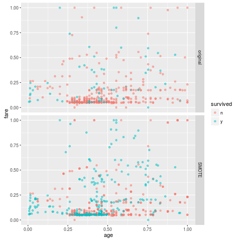
Method 1) SMOTE

SMOTE one of over sampling methods and it generates samples in an artificial way. The package DMwR contains a function which provides the implementation.

library(DMwR)
set.seed(11)
df.sm <- df.train %>% mutate(survived=as.factor(survived))
df.sm <- SMOTE(survived~., df.sm, perc.over=288,k=2) ### applying SMOTE algorithm

While the original training contains only 81 positive samples, the data set after SMOTE contains 243 positive samples. The positive rate has become around 43%. (I set perc.over so that the size of the positive samples becomes 3 times.)

> table(df.train$survived) ### original training set
  n   y 
314  81 
> table(df.sm$survived) ### after SMOTE
  n   y 
324 243 

Note that the number of negative samples has slightly been increased.

The training result is following.

     method acc.train  acc.test    y.rate    recall precision  F1.score
1    nobody 0.7949367 0.7938931 0.0000000 0.0000000 0.0000000 0.0000000
2    glmnet 0.7721519 0.7709924 0.2519084 0.5555556 0.4545455 0.5000000
3 svmRadial 0.7797468 0.7404580 0.3129771 0.6296296 0.4146341 0.5000000
4        rf 0.9265823 0.7328244 0.2977099 0.5740741 0.3974359 0.4696970
5   xgbTree 0.8911392 0.7328244 0.3206107 0.6296296 0.4047619 0.4927536

Comparing with other sampling methods which we used in the last entry, the F1 scores are slightly better. We note that the result largely depends on the choice of prec.over.

Method 2) Ensemble method

One of the disadvantage of under sampling is that we just ignore many negative samples. That is, we do not use the ignored negative samples if we apply the under sampling method. To reduce the number of ignored samples, we may use multiple under-sampled training sets.

The logic is easy to understand. We generate $k$ training sets $X_1, \cdots, X_k$ by under sampling. We train models $\hat f_1, \cdots, \hat f_k$ on the training sets. Given a sample $x$, we take the sum $\hat f_1 (x) + \hat f_k (x)$. The larger the sum is, the more it is likely to be positive. To make an explicit prediction we have to choose a threshold $t$, i.e. if the sum $\geq t$, then the sample is predicted as a positive sample. (The implementation can be found on this repository. We do not show it be cause it is quite long to put on a blog entry.)

Following the logic, we can think that a largeer $k$ is better, but this is wrong. You can find the reason by looking at the result for the case when $k=3$:

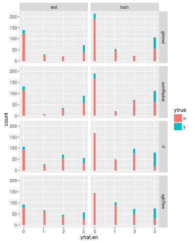
The x-axis shows that the sum. Note that the result on the test set lies on the left hand. As you see in the histogram, the positive samples are distributed for all bin. Therefore we have to choose $t = k$.

There is another problem: the behaviors of the trained models are quite different. (For example the recall of glmnet is high, while one of random forest is relatively small.)

     method     yrate  accuracy    recall precision  F1.score
1    glmnet 0.2748092 0.7786260 0.6296296 0.4722222 0.5396825
2 svmRadial 0.3396947 0.6984733 0.5925926 0.3595506 0.4475524
3        rf 0.2137405 0.7480916 0.4074074 0.3928571 0.4000000
4   xgbTree 0.2175573 0.7900763 0.5185185 0.4912281 0.5045045

For the case where $k=2$ is following:

     method     yrate  accuracy    recall precision  F1.score
1    glmnet 0.2786260 0.7748092 0.6296296 0.4657534 0.5354331
2 svmRadial 0.3664122 0.7022901 0.6666667 0.3750000 0.4800000
3        rf 0.2938931 0.7213740 0.5370370 0.3766234 0.4427481
4   xgbTree 0.2938931 0.7595420 0.6296296 0.4415584 0.5190840

Note that the case $k=1$ is just an under sampling method we saw in the last entry. The following is just a copy from the previous entry.

     method acc.train  acc.test    y.rate    recall precision  F1.score
1    nobody 0.7949367 0.7938931 0.0000000 0.0000000 0.0000000 0.0000000
2    glmnet 0.7367089 0.7251908 0.3282443 0.6296296 0.3953488 0.4857143
3 svmRadial 0.7113924 0.6793893 0.3969466 0.6851852 0.3557692 0.4683544
4        rf 0.7468354 0.6717557 0.3740458 0.6111111 0.3367347 0.4342105
5   xgbTree 0.7620253 0.7137405 0.3473282 0.6481481 0.3846154 0.4827586

So we may see the ensemble method is better than the only one under sampling. But to be honest it is not worth trying an ensemble model because it cannot defeat SMOTE (at least this time). (But the performance of elasticnet (glmnet) becomes slightly better.)