In the last entry we looked at the imbalanced classification problems. In this entry we try sampling methods and observe what happens.

NB: We show only part of code and the result. The complete code can be found my BitBucket repository.

Data

We use the famous Titanic data. If you have tried a famous competitoin, you must know that most of men died. That is the "survived" variable is skewed after restricting the data to male samples. We can find the data in PASWR package.

library(caret); library(ggplot2); library(plyr); library(dplyr); library(tsne)
library(ROSE) ## library for sampling methods

df <- PASWR::titanic3 %>% 
    filter(sex=='male') %>%
    select(-name,-sex,-ticket,-boat,-body,-home.dest) %>%
    mutate(cabin=ifelse(cabin=='',1,0),
           survived=ifelse(survived==1,'y','n'))

For simplicity we use the complete rows (i.e. ignore samples containing NA, etc.). We split the data into a training set and a test set:

set.seed(1)
in.train <- createDataPartition(df$survived,p=0.6,list=F)
df.train <- slice(df,in.train) ## 395 samples
df.test <- slice(df,-in.train) ## 262 samples

Looking at the training data, we normalize the data and the result looks like the following

> set.seed(2)
> sample_n(df.train,5)
    pclass survived       age sibsp     parch       fare cabin    embarked
74       1        y 0.6923077   0.2 0.3333333 0.89666667     0   Cherbourg
277      0        n 0.4307692   0.4 0.0000000 0.05283333     1 Southampton
226      0        n 0.3230769   0.0 0.0000000 0.05155533     1  Queenstown
66       1        n 0.9384615   0.2 1.0000000 1.00000000     0   Cherbourg
370      0        y 0.4769231   0.0 0.0000000 0.05283333     1 Southampton

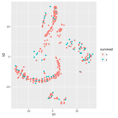
In the training set the rate of survived samples around 20.5%. Thus the useless model "no survived samples" achieves around 80% accuracy. If we project the data into 2-dimensional with t-SNE, the data looks like:

Sampling methods

Before applying sampling methods we check performance of honest statistical models:

     method acc.train  acc.test     y.rate    recall precision  F1.score
1    nobody 0.7949367 0.7938931 0.00000000 0.0000000 0.0000000 0.0000000
2    glmnet 0.8025316 0.8282443 0.04961832 0.2037037 0.8461538 0.3283582
3 svmRadial 0.7949367 0.7938931 0.00000000 0.0000000       NaN       NaN
4        rf 0.8531646 0.8206107 0.04961832 0.1851852 0.7692308 0.2985075
5   xgbTree 0.8253165 0.8282443 0.08015267 0.2777778 0.7142857 0.4000000

"nobody" is the useless model. The XGBoost model is the best among the above methods. But we should note that the rate of 'y' and the recall are both very low.

We use ROSE package to apply sampling methods.

Undersampling

Roughly speaking, the undersampling ignores part of "negative" samples so that the number of the negative samples is near to the number of the positive samples.

df.us <- ovun.sample(survived~.,data=df.train, method="under",
                     N=2*sum(df.train$survived=='y'),
                     seed=3)$data

While the original training set df.train contains 314 negative samples and 81 positive samples, the numbers of negative and positive samples in the undersampled data set df.us are both 81.

     method acc.train  acc.test    y.rate    recall precision  F1.score
1    nobody 0.7949367 0.7938931 0.0000000 0.0000000 0.0000000 0.0000000
2    glmnet 0.7367089 0.7251908 0.3282443 0.6296296 0.3953488 0.4857143
3 svmRadial 0.7113924 0.6793893 0.3969466 0.6851852 0.3557692 0.4683544
4        rf 0.7468354 0.6717557 0.3740458 0.6111111 0.3367347 0.4342105
5   xgbTree 0.7620253 0.7137405 0.3473282 0.6481481 0.3846154 0.4827586

The precision becomes smaller, but the recall is so improved that the F1 score also becomes better. In particular SVM works after the undersampling. Namely the positive samples are no longer minority (or "outliers") in df.us.

One of the disadvantage of the undersampling is that we do not use relatively large number of negative samples. That must be one of the reasons for the large yrate and recall. Namely the trained models fail to detect negative samples as negative samples.

Oversampling

The oversampling duplicates positive samples. Thus we use all negative samples in comparison with undersampling.

df.os <- ovun.sample(survived~.,data=df.train,method="over",
                     N=2*sum(df.train$survived=='n'),
                     seed=4)$data

The oversampled training set contains 314 negative samples and 314 positive samples. Since the actual number of positive samples is 81, each positive sample appears 3.87 times in df.os on average.

     method acc.train  acc.test    y.rate    recall precision  F1.score
1    nobody 0.7949367 0.7938931 0.0000000 0.0000000 0.0000000 0.0000000
2    glmnet 0.7113924 0.7099237 0.3511450 0.6481481 0.3804348 0.4794521
3 svmRadial 0.7772152 0.7404580 0.2900763 0.5740741 0.4078947 0.4769231
4        rf 0.9848101 0.7519084 0.2328244 0.4629630 0.4098361 0.4347826
5   xgbTree 0.9518987 0.7442748 0.2480916 0.4814815 0.4000000 0.4369748

In comparison with undersampling, the predicted rate of "y" is smaller, but it is still larger than the actual positive rate (i.e. around 0.2). The recall is slightly smaller but the precision is improved so that there is no remarkable difference of F1-scores.

We should note that the size of the training set becomes relatively large after the oversampling. While the original training set consists of 395 samples, df.os consists of 628 samples.

Applying both undersampling and oversampling

df.both <- ovun.sample(survived~.,data=df.train,method='both',N=400,seed=5)$data

The data frame df.both contains 214 negative samples and 186 positive samples.

     method acc.train  acc.test    y.rate    recall precision  F1.score
1    nobody 0.7949367 0.7938931 0.0000000 0.0000000 0.0000000 0.0000000
2    glmnet 0.7468354 0.7175573 0.3206107 0.5925926 0.3809524 0.4637681
3 svmRadial 0.7696203 0.6946565 0.3282443 0.5555556 0.3488372 0.4285714
4        rf 0.8607595 0.6908397 0.3549618 0.6111111 0.3548387 0.4489796
5   xgbTree 0.8481013 0.6984733 0.3167939 0.5370370 0.3493976 0.4233577

The result can depend on the number of samples N and the proportion p of the positive class. (The default is p=0.5.) But our result is similar to the result of the undersampling.

Next Entry

The undersamplings and oversamplings are both very easy to understand. In the next entry we try slightly complicated method for a imbalanced classification model.

Tips

• You might improve either recall or precision by adjusting the size of the sampled data. (That is the N option in the ovun.sample().)
• As we mentioned in the first entry, we rely on the caret package for turning meta parameter. That is because the goal of an imbalanced classification problem is not necessarily the high accuracy. So the choice of meta parameters depends on the question. Moreover the aim of this entry is an observation of the sample methods, not the careful turning for the data set. But we have to choose meta parameters, so we let caret choose them.