

Arrow::LogisticRegression
A logistic regression classifier is now available in the Perl module Arrow. Its usage is very similar to LogisticRegression in scikit-learn.
I have written two scripts in Perl and Python for comparison: plr-multinomial.pl and plr-multinomial.py. In the scripts we use 'iris.csv'. This is a famous dataset and we can create it by the following command.
bash$ R --quiet -e "write.csv(iris,'iris.csv')"
The Perl script is following:
#!/usr/bin/perl
use strict;
use warnings;
use utf8;
use 5.010; # only for "say"
use PDL; # this module corresponds to NumPy of Python.
use Arrow::DataFrame; # import the Perl module for data frames
use Arrow::Model qw(LogisticRegression); # Logistic regression classifier

my $df = Arrow::DataFrame->read_csv('iris.csv')->select('-0');
say "Our data (iris.csv):";
$df->show(head=>5,width=>12); # show the first 5 observations in the dataset
print "Hit the enter key: "; <>;
The variable $df is a data frame of the iris dataset. select('-0') deletes the first column from the imported dataset, because the column is just observation IDs.
Our data (iris.csv):
    | Sepal.Length | Sepal.Width  | Petal.Length | Petal.Width  | Species
000 | 5.1          | 3.5          | 1.4          | 0.2          | setosa
001 | 4.9          | 3            | 1.4          | 0.2          | setosa
002 | 4.7          | 3.2          | 1.3          | 0.2          | setosa
003 | 4.6          | 3.1          | 1.5          | 0.2          | setosa
004 | 5            | 3.6          | 1.4          | 0.2          | setosa
Hit the enter key:
After the enter key is hit, the following code is executed.
my $y = $df->cols('Species'); # an arrayref of the target variable (not a piddle)
my $X = $df->select('-Species')->as_pdl; # $X must be a piddle
The design matrix $X is require to be a piddle (a PDL object) but the target variable $y is not. (Note that a piddle is not able to contain non-numerical data such as a string.)
my $cw = {setosa=>1,versicolor=>2,virginica=>3}; # class_weight
my $plr = LogisticRegression(lambda=>1,class_weight=>$cw); # classifier instance
$plr->fit($X,$y); # fit
We can assign class weights by a hash (reference). Thanks to good numerical performance of PDL, the training process finishes in a very short time.
say "Predicted Probabilities:";
print "classes: ",join "    ", @{$plr->classes}; # classes
my $predict_proba = $plr->predict_proba($X); # predict probabilities
print $predict_proba;
predict_proba() method predicts probabilities of classes for each observation. Using classes()-method we can check which column corresponds to which class. In this script $plr->classes is an arreyref ['setosa','versicolor','virginica'] and the first column of $predict_proba corresponds the class "setosa".
say "intercepts: ", $plr->intercept_;
print "coef: ", $plr->coef_;

print "accuracy on train: ";
my $prediction = $plr->predict($X);
say avg(pdl map { $y->[$_] eq $prediction->[$_] } 0..($df->nrow()-1));
exit;
The above codes shows the estimated parameters and the accuracy of the predictive model on the training set. You can find that the result of our Perl script is the same as one of scikit-learn.
Technical details
Our implementation follows Park-Hastie [1]. I added partial function of "class_weight" of scikit-learn. Note that class_weight='balanced' has not been implemented yet.
We create a "one-versus-rest" classifier. Suppose that the target variable takes $0, \cdots, K-1$ and consider a classifier of the class $k \in \lbrace 0,\cdots,K-1 \rbrace$. Our cost function is defined by
$$J_k(\beta) = \sum_{i=1}^n w(g^i) \Bigl( I(g^i \ne k)\log(1-\sigma(\langle\beta,x^i\rangle)) + I(g^i=k) \log\sigma(\langle\beta,x^i\rangle) \Bigr) + \frac{\lambda}{2}\|\beta'\|^2$$
Here $g^i$ ($=0,\cdots,K-1$) is the class of the i-th observation, $w(g^i)$ is a class weight of the class $g^i$, $\sigma$ is the sigmoid function: $\sigma(z) := 1/(1+\exp(-z))$, $\lambda$ is a penalty coefficient and $\beta' = (0,\beta_1,\cdots,\beta_p)$. ($\beta_0$ is the intercept.)
Because of the formula of the cost function, A multiplication of class weights and a (positive) constant $c$ has the same effect as replacement of $\lambda$ with $\lambda/c$.
Remark. In scikit-learn we use C instead of $\lambda$. The relation between them is $C=1/\lambda$.
Let $p_0(x), \cdots, p_{K-1}(x)$ be trained predictive models. The sum $s(x) := p_0(x) + \cdots + p_{K-1}(x)$ must be 1, but there is no a priori reason that the equation holds. Therefore we normalise the predictive values. Namely $p_k(x)/s(x)$ is the estimate of $\mathbb P(Y=k|X=x)$.
Optimisation Method
The Newton-Raphson method is implemented as an optimisation method. Therefore if the number of predictors is very large, then it takes quite long time to train the model (because of the inverse of Hessian). I will probably implement L-BFGS someday, but not "liblinear" [2].
One-versus-rest classifier
Even in the binary classification our classifier construct a one-versus-rest classifier. This is completely a waste of resources because of the following reason. Let $p_0(x)$ and $p_1(x)$ be predictive models for the class 0 and 1, respectively. Then we can observe that $p_0 + p_1 \equiv 1$ holds. This is because the symmetry $1-\sigma(z) = \sigma(-z)$ implies $J_0(\beta) = J_1(-\beta)$. Namely the regression coefficient of the class 1 is the opposite sign of one of the class 0.
Data Experiment: why we need Newton-Raphson method
Let us try a very easy example of logistic regression. Our dataset "plr.csv" can be found at the usual repository. There is only one predictor $x$ and a binary target variable $y$. The scatter plot is following.
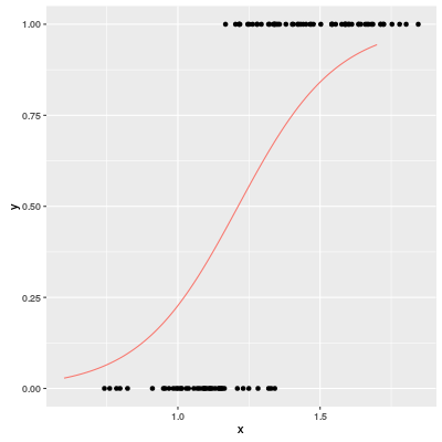
The red graph is a predicted probabilities of a logistic regression model ($\lambda=0.5$).
The gradient descent is the most famous optimization method. But it is not a good idea to use it for logistic regression because of the graph of a cost function.
If you execute "plr.pl", you can check the result of Newton-Raphson method and the gradient descent. The first data frame is the result of Newton-Raphson.
    | c        | b        | cost
000 | 0        | 0        | 68.62157
001 | -5.45281 | 4.450280 | 41.95503
002 | -6.83869 | 5.633772 | 40.72107
003 | -6.99932 | 5.776966 | 40.70540
004 | -7.00144 | 5.778930 | 40.70540
"c" is the intercept and "b" is the regression coefficient for x: $\beta = (c,b)$. The Newton-Raphson method is terminated after 5 steps. The value of he cost function reaches 40.7.
On the other hand the gradient descent can not reach even 45 after 100 steps. Namely the gradient descent is not efficient for logistic regression.
    | c        | b        | cost
096 | -4.62404 | 3.913047 | 46.74198
097 | -4.63300 | 3.919850 | 46.73841
098 | -4.64176 | 3.926429 | 46.73503
099 | -4.65027 | 3.932873 | 46.73182
100 | -4.65857 | 3.939118 | 46.72877
Looking at the following diagram, we can easy understand this phenomenon.
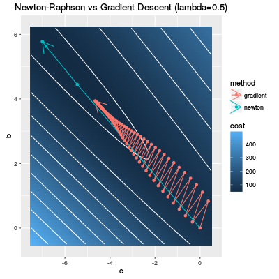
The white curves are contour curves of the cost function and the darker blue means lower cost. If you have learnt the gradient descent, you know an example where the gradient decent does not work. Our cost function is exactly such a function.
The red curve shows the change of the parameter by gradient descent and it is easy to see that the gradient descent steps are not efficient. On the other hand the Newton-Raphson method (the blue curve) is so efficient that the parameter goes in a dark blue region only in a few steps.
Our dataset is not a special case: the cost function of a logistic regression is likely to have a graph like our cost function. That is because the cost function is basically a sum of functions of form $\mathrm{cost}(z) = -\log(\sigma(z))$ and its graph is following
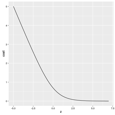
Therefore the gradient of a cost function is very small in the region where the cost function takes small values.
References
- Mee Young Park and Trevor Hastie. Penalized logistic regression for detecting gene interactions. 2008.
- Lin Chih-Jen, Ruby C. Weng, and S. Sathiya Keerthi. Trust region Newton method for large-scale logistic regression. 2008.