Quick Reference for R [c r e s c e n t]

Quick Reference for R

Last Modified: 2017-06-17

The aim of this document is to provide grammar and examples of R commands so that I remember keywords (e.g. names of packages) and details (options, etc).

Instead of the most general description, typical examples are provided. One of its conclusion is that some functions can be applied to other objects. Ex. x of sequence(x) could be a vector, but only sequence(10) is given in this document.

Disclaimer

At your own risk.
This is NOT a complete list of options. See manual for it.

Versions

CRAN provides a repository for R packages, which are newer than ones on the official repository of openSUSE. Therefore we use packages of CRAN. (At the page: "Download R for Linux" → "suse".)

sessionInfo() shows the versions of R and loaded packages.

R version 3.2.2 Patched (2015-10-23 r69569)
Platform: x86_64-suse-linux-gnu (64-bit)
Running under: openSUSE (x86_64)

Manual, Tutorial, etc

The R-Manuals, Quick-R, R Tutorial, Wikibooks (de), Cookbook for R
Data Science Specialization, An Introduction to Statistical Learning, Computing with Data Seminar
Cheatsheets by RStudio including ggplot2, dplyr and R Markdown
How to set the default mirror for packages.
If the error system(full, intern = quiet, ignore.stderr = quiet, ...) happens for installing a package, then options(unzip = 'internal') might solve the problem.

Data type

Atomic classes: integer, numeric, character, logical, complex. Let atomic be one of them.

class(x) find a class of x
is.atomic(x): if x is atomic, then "T".
integer(length=3) : an initialised vector c(0,0,0). "integer" can be one of the above classes.
as.factor(x) : convert x into factor. "factor" can be one of the atomic classes.

Character

substr("abcde",2,4): "bcd"
strsplit("abc|def|ghi","|",fixed=T) : gives list(c("abc","def","ghi"))
paste("X",1:5,sep="."): "X.1" "X.2" "X.3" "X.4" "X.5"
paste(c("a","b"),c("x","y"),sep="."): "a.x", "b.y"
paste(c("a","b","c"), collapse=" "): "a b c".
paste0(x) : equivalent to paste(x,sep="").
sprintf(fmt="%03d",1): "001".

Regular Expression

Tutorial.

grep(pattern,vec,...) searches the pattern in a vector. value=F (default) gives the indices of matched elements and value=T gives the matched elements. Do not forget to escape backslashes in a regular expression.

vec <- c("abc1234", "de23f", "gh3ij", "45klmn67")
grep("\\d\\d", vec, value=F) ## 1, 2, 4
grep("\\d\\d", vec, value=T) ## "abc1234", "de23f", "45klmn67"
grepl("\\d\\d", vec)         ## T, T, F, T (boolean)

regexpr() gives an integer vector consisting of the position of the matched part. The vector has also attribute match.length consisting of the length of matched part.
```
vec <- c("abc1234", "de23f", "gh3ij", "45klmn67")
match <- regexpr('\\d\\d', vec, perl=T)
match                      ## 4  3 -1  1
attr(match,'match.length') ## 2  2 -1  2
```
regmatches() gives the matched part. (Be careful about the length of the output!)
```
regmatches(vec, match) ## "12", "23", "45"
```
This function accept substitution. But for this purpose we should use sub instead.

sub(pattern,subst,vect) replaces the matched part with a new string. gsub() is the global version of sub().

vec <- c("abc1234", "de23f", "gh3ij", "45klmn67")
sub('(\\d\\d)',"[\\1]",vec)  ## "abc[12]34",   "de[23]f", "gh3ij", "[45]klmn67"
gsub('(\\d\\d)',"[\\1]",vec) ## "abc[12][34]", "de[23]f", "gh3ij", "[45]klmn[67]"

Logical

!, &, |, xor(,): NOT, AND, OR, XOR. (These are component-wise.)
&&, ||: details.
isTRUE(x): if x is T, then T, else F.

Factor

factor(c(1,2,2,3,3,3)): make the input a vector of factors. (Levels: 1 2 3)
levels(factor(c(1,2,2,3,3,3))): "1","2","3". The character vector of the factors
table(factor(c("a","b","b","c","c","c"))): counts the elements for each factor.

Hmisc

cut2() make a factor variable of intervals from a numerical variable
cut2(vec,g=3): divide range(vec) into 3 intervals

Date and Time

References : Tutorial1, Tutorial2 (PDF), Date Formats in R.
library(lubridate) : see GitHub, Dates and Times Made Easy with lubridate

Date objects

today <- Sys.Date() ## today "2015-01-24" (Date object)

as.Date("12.08.1980",format="%d.%m.%Y") : string → Date object
as.Date(3,origin="2015-01-01") : 3 days after of "origin", i.e. "2015-01-04".
as.Date(0:30,origin="2015-01-01"): vector of Date objects (of January 2015).
seq.Date(from=date1,to=date2,by="day") : similar to the above. (Date objects are required.)

POSIXct/POSIXlt objects

now <- Sys.time()           ## "2015-01-24 12:19:24 CET" (POSIXct object)
cat(now,"\n")               ## 1422098364
as.POSIXlt(now)$year + 1900 ## 2015

Sys.time(): gives the current time in POSIXct. Ex "2015-08-25 23:55:59 CEST".
strptime("2015-01-02 03:04:05",format="%Y-%m-%d %H:%M:%S") : string → POSIXlt

There are two basic classes of date/times.

POSIXct : the (signed) number of seconds since the beginning of 1970 (in UTC)
POSIXlt : a list of vectors consisting of sec, min, hour, mday, mon (0–11), year (years since 1900), wday (0(Sun)–6(Sat)), yday (0–365), and isdst. Namely the R-version of localtime()-format.
dplyr can not handle POSIXlt format. Thus it is better to stick with POSIXct format.

Manipulate

We can compare two Date/POSIXct/POSIXlt objects.
- past < today is TRUE, past > today is FALSE.
- today - past : the date difference. Don't forget as.numeric() to get the result as a number.
- difftime(today,past,units="secs") : time difference in seconds.

format(today, format="%B %d %Y"): Date object → string

dates <- format(as.Date(0:20,"2016-01-01")) ## vector of strings of dates
dates[2]                                    ## 2016-01-02 (2nd entry)
match("2016-01-14",dates)                   ## 14 (the num. of the entry)

(This idea comes from "Tutorial2" above.)

Vector

The R-version of an array. The index starts from 1 (not 0).

x = c("b","d","a","c","e")
x[1]  ## "b"
x[-1] ## "d" "a" "c" "e" (Remove the first element.)

1:10 or sequence(10) : 1, 2, 3, 4, 5, 6, 7, 8, 9, 10. (Different from Python's range()!)
length(1:10) : 10
seq(0,1,length=5): 0.00, 0.25, 0.50, 0.75, 1.00
rep("a",5): "a", "a", "a", "a", "a"
rep(1:2,3): 1, 2, 1, 2, 1, 2
rep(1:2,each=3) : 1, 1, 1, 2, 2, 2

As a set

unique(c("a","b","b","c","c","c")) : "a", "b", "c". Remove the duplicate elements.
union(1:3,2:4): 1,2,3,4. The union ∪
intersect(1:7,5:10): 5,6,7. The intersection ∩
setdiff(1:7,5:10) : 1, 2, 3, 4. The set difference.
1:2 %in% 2:5 : F, T. The ∈ operator.
range(1:8,5:12,na.rm=F): 1, 12. The vector representing the range of the vectors.

Manipulation

1:5 > 2: F, F, T, T, T
x[1:5>2]: x[3], x[4], x[5]. Pick the elements corresponding to TRUE.
x[c(3:5)]: x[3], x[4], x[5]. Pick the 3rd–5th elements.
x[c(-1,-2)], x[-c(1,2)], x[-(1:2)]: x[3], x[4], x[5]. Remove the 1st and 2nd elements.

Sort

x = c("b","d","a","c","e")
sort(x)              ## a, b, c, d, e (ascending order)
sort(x,decreasing=T) ## e, d, c, b, a (descending order)

The order() command sorts the index by looking at the entries of the vector.

order(x) ## 3, 1, 4, 2, 5

This means that c(x[3],x[1],x[4],x[2],x[5]) is the sorted vector:

x[order(x)] ## a, b, c, d, e (ascending order)

We can use order() to sort a vector with respect to another vector:

attend <- c('Alice','Bob','Cris','David')
scores <- c( 80,     70,   90,    60)
attend[order(scores,decreasing=T)] ## Cris, Alice, Bob, David (desc. order of scores)

List

lst <- list(a="X",b=1:3): lst[[1]]==lst$a=="X" and lst[[2]]==lst$b==c(1,2,3).
labels(list(a=1,b=2)): "a", "b".

Table

x <- c('a','a','a','b','b','c')
table(x) ## count the values in the vector
## x
## a b c 
## 3 2 1

table(vec1,vec2) : the confusion matrix.
prop.table(): Express Table Entries as Fraction of Marginal Table

Data frame

A data frame consisting of

$p$ vectors with the same length $n$. ($n$ = nrow, $p$ = ncol)
a name of each column (names)
indexes of rows (row.names)

	col1	col2	col3
1	4	a	TRUE
2	5	b	TRUE
3	6	a	FALSE
4	7	b	FALSE

The above data frame can be constructed as follows.

vec1 <- 4:7
vec2 <- rep(c('a','b'),2)
vec3 <- rep(c(T,F),each=2)
df <- data.frame(col1=vec1,col2=vec2,col3=vec3)
nrow(df)      ## 4                (number of rows)
ncol(df)      ## 3                (number of columns)
dim(df)       ## 4,3              (nrow(df), ncol(df))
names(df)     ## col1, col2, col3 (the vector of the names of columns)
row.names(df) ## 1,2,3,4          (the vector of row indexes)

names(df) accepts a substitution to change a colunm name.
df$col4 <- vec4 add a new column "col4" with values of "vec4".

Look at a data frame

str(df) : show the type and first several elements of each column
summary(df): statistical summary of each column

	`df$col1`, `df[,1]`/`df[1]`	`df$col2`/`df[2]`	`df$col3`/`df[3]`
`df[1,]`	`df[1,1]`	`df[1,2]`	`df[1,3]`
`df[2,]`	`df[2,1]`	`df[2,2]`	`df[2,3]`
`df[3,]`	`df[3,1]`	`df[3,2]`	`df[3,3]`
`df[4,]`	`df[4,1]`	`df[4,2]`	`df[4,3]`

The following slices accept a substitution to change the values.

Columns

While df$col1 and df[,1] are vectors, df[1] is the data frame consisting only of the first column.
df[integer vector] / subset(df,select=integer vector) gives a data frame consisting of the specified columns. Do not forget that a negative integer means removing.
df[boolean vector] gives a data frame consisting of columns corresponding to T.
Do not forget select() of dplyr.

Rows

df[1,] is the data frame consisting only of the first row. (However df[,1] is a vector.)
df[integer vector,] gives a data frame consisting of the specified rows. (Do not forget ,!)
df[boolean vector,] / subset(df, boolean vector) gives a data frame consisting of rows corresponding to T.
Do not forget filter() and slice() of dplyr.

Manipulation

df <- rbind(df, list(10,"a",T)) : add a row (or a data frame) at the bottom.
df <- cbind(df, list(col4=vec4)) : add a column (or a data frame).
df <- transform(df, col4=vec4): add a column.
df <- transform(df, col1=factor(col1)): convert the class of a column
unique(df) : remove duplicate of rows.
Do not forget distinct() and mutate() of dplyr.

apply family

This section is not only for data frames.
func is a function. We can define a function with function(x) { ... }.
lapply(vec,func) : list of results applying each element of x to the function f.
sapply(X,func) : similar to lapply(). But the result is a vector or a matrix (or an array).

tapply(vec,grp,func) is something like 'groupby' for vectors.

vec <- 1:10                   ## 1, 2, 3  4  5    6  7  8  9, 10
grp <- rep(c('a','b'),each=5) ## a, a, a, a, a,   b, b, b, b, b 
tapply(vec,grp,mean)
## a b 
## 3 8

apply(X,1,func) applies a function to each row and gives a result as a vector.
apply(X,2,func) applies a function to each columns and gives a result as a vector.
Here X is a matrix or a data frame.

Merge

merge(x=df1,y=df2,by="col1"): merge two data frames (by glueing along col1)
- Use by.x and by.y to glue along the different column names.
merge(df,dg,by=NULL) : cross join
merge(df,dg,all=T) : outer join
merge(df,dg,all.x=T) : left join (keep all rows for df)
merge(df,dg,all.y=T) : right join (keep all rows for dg)

Dealing with missing values

apply(df,1,function(x) sum(is.na(x))) counts the number of NA in each column.
complete.cases(df): TRUE, TRUE, TRUE, TRUE. Whether is the row complete.

reshape2

An introduction to reshape2: reshape2 is an R package written by Hadley Wickham that makes it easy to transform data between wide and long formats.

dg <- data.frame(a=11:14,b=rnorm(4),c=rep(c("A","B"),2))
melt(dg,id=c("a"),measure.vars=c("b","c"))
##    a variable             value
## 1 11        b  1.22408179743946
## 2 12        b 0.359813827057364
## 3 13        b 0.400771450594052
## 4 14        b  0.11068271594512
## 5 11        c                 A
## 6 12        c                 B
## 7 13        c                 A
## 8 14        c                 B

melt makes a wide data frame a long one. dcast makes a long data frame a wide one.

dcast(dh, a~variable, value.var="value")
##    a                 b c
## 1 11  1.22408179743946 A
## 2 12 0.359813827057364 B
## 3 13 0.400771450594052 A
## 4 14  0.11068271594512 B

plyr

Use dplyr instead.
A tutorial with sample data and A quick introduction to plyr (pdf).

dplyr

See the cheatsheet by RStudio or Introduction to dplyr. This section is a brief summary of the latter.

The dplyr packages converts each data frame into an object of tbl_df class to prevent huge data from beeing printed.
The output is always a new data frame.
For the following functions we may write x %>% f(c) instead of f(x,c). This notation is convenient if we need to compose several functions.

filter()

This gives the subset of observations satisfying specified conditions.

filter(df,col1==1,col2==2)

is the same as df[df$col1==1 & df$col2==2,]. We can use boolean operators such as & or |:

filter(df,col1==1|col2==2)

If you want to get a subset of observations in a random way, then we may use the following functions.

sample_n(df,10) : pick up 10 observations randomly
sample_frac(df,0.6) : pick up 60% of the observations randomly

arrange()

This rearranges the observations by looking at the specified variables.

arrange(df, col3, col4)

is the same as df[order(df$col3,df$col4),] (i.e. in ascending order). Use desc() to arrange the data frame in descending order.

arrange(df, desc(col3))

select()

This returns a subset of the specified columns.

select(df,col1,col2)

is the same as subset(df,select=c("col1","col2")). We can use : to specify multiple columns. Namely

select(df, col1:col3) ### same as subset(df,select=c("col1","col2","col3"))

We can also use - to remove the column.

select(df, -col1) ### same as subset(df,select=-col1)

distinct() is sometimes used with select() to find out the unique (pairs of) values.

rename()

This changes the name of the column.

rename(df, newColName=oldColName)

mutate()

This adds a new column to the data frame, following the specified formula.

mutate(df, newCol1 = col1/col2, newCol2=col3-3*col4)

If you want the data frame with only the new columns, then use transmute instead.

summarise()

This generates summary statistics of specified variables.

summarise(df,meanCol1=mean(col1),sdCol2=sd(col2))

The output is a data frame consisting of only one row.

The functions which can be used in summarise() (mean and sd in the above expample) must be aggregate functions, i.e. they send a vector to a number. So we may use min(), sum(), etc. Moreover the following functions are available.

n(): the number of observations in the current group
n_distinct(x) : the number of unique values in x.
first(x) (==x[1]), last(x) (==x[length(x)]) and nth(x,n) (==x[n])

group_by()

byCol1 <- group_by(df,col3)

The result is a "map" sending a value v in col3 to a data frame select(df,col3==v). Then we can apply the above functions to byCol1.

Data.Table

This section is not finished.

data.table provides a faster version of a data frame.
- The website including "Getting started".
- The difference between data.frame and data.table.

Mathematics

Functions

pi==3.141592
round(pi,digits=2)==3.14, round(pi,digits=4)==3.1416
sin(), cos(), tan(), asin(), acos(), atan(), log(), log10(), log2(), exp(), sqrt(), abs(), ceiling(), floor()
atan2(y,x) : $\arg(x+\sqrt{-1}y)$ in $(-\pi,\pi]$.
sum(vec,na.rm=F), prod(vec,na.rm=F): take the sum/product of elements.

Matrix

A <- matrix(data=1:6,nrow=2,ncol=3,byrow=F); A
     [,1] [,2] [,3]
[1,]    1    3    5
[2,]    2    4    6

t(A): transpose matrix.
diag(A): 1, 4. The diagonal part of a matrix.
A %*% B: matrix product.
solve(A): inverse matrix.
solve(A,b): solution to $Ax=b$.
which(A>4,arr.ind=T): matrix indicating the entries satisfying the condition.

Probability Theory

Let $X:\Omega\to\mathbb R$ be a random variable on a probability space $(\Omega,\mathcal A,\mathbb P)$.
$\Phi(x) := \mathbb P(X \leq x)$ : (cumulative) distribution function (cdf)
$q_\alpha := \Phi^{-1}(\alpha)$: quantile function
$\phi := d\Phi/dx$: probability density function (pdf) (The density of the pushforward $X_*\mathbb P$.)

Normal Distribution

rnorm(n,mean=0,sd=1): random generation for the normal distribution. (n : how many)
pnorm(x,mean=0,sd=1) : cdf
qnorm(alpha,mean=0,sd=1) : quantile function
dnorm(x,mean=0,sd=1): pdf

Similar functions are supported for some other distributions.

dbinom(n, size, prob): $\mathbb P(X=k) = {}_nC_k p^k (1-p)^{n-k}$ (Binomial)
dpois(x, lambda) : $\mathbb P(X=k) = e^{-\lambda}\lambda^k/k!$ (Poisson)
dexp(x, rate=1): $\phi(x) = 1_{ x > 0 }\lambda e^{-\lambda x}$ (exponential)
dunif(x,min=0,max=1): $\phi(x) = 1_{x \in (0,1) }$ (uniform)

Statistics

This section has not been written yet.

max(), min(), mean(), sd(), var(), median(). Note that na.rm=F is the default setting.
cor(vec1,vec2) correlation
sample(1:3,10,replace=T): construct a sample of length 10 from 1:3. Ex. 2, 3, 1, 1, 3, 3, 2, 2, 1, 3.
sample(vec) : shuffle the entries of the vector randomly.

Hypothesis Testing

$\lbrace \mathbb P_\theta \ |\ \theta \in \Theta \rbrace$ : a statistical model
$\Theta = \Theta_0 \sqcup \Theta_1$ : disjoint union
H₀ : $\theta \in \Theta_0$ : Null Hypothesis
H_A : $\theta \in \Theta_1$ : Altenative Hypothesis

	Null Hypothesis (H₀)	Alternative Hypothesis (H_A)
Accept Null Hypothesis	True Negative	False Negative (Type 2 error)
Reject Null Hypothesis	False Positive (Type 1 error)	True Positive

We often decide to accept or reject the null hypothesis by using a test statistic $T$.

$$\delta(X) = \begin{cases} 0\ \text{(accept)} & \text{if}\quad T(X) \geq c \\ 1\ \text{(reject)}& \text{if}\quad T(X) < c \end{cases} $$

We choose a test statistic so that the significance level $\alpha := \sup_{\theta \in \Theta_0} \mathbb P_\theta(\text{Reject})$ is small.

The p-value, defined by $\sup_{\theta \in \Theta_0} \mathbb P_\theta(T(X) \geq T(x) )$, is the largest probability under the null hypothesis that the value of the test statistic will be greater than or equal to what we observed.

Kolmogorov-Smirnov test (KS-test)

The KS test is used to compare the distributions of two random variables. Given $F_X$ and $F_0$ be two cumulative distribution functions, then our hypothesis test is:

Null hypothesis : $F_X = F_0$.
Alternative hypothesis : $F_X \ne F_0$.

Such a hypothesis test is often used to see whether the distribution of a variable $X$ is normal/Bernoulli/etc. Namely $F_X$ is the CDF of $X$ and $F_0$ is the CDF of a normal distribution. Therefore we consider only such a situation.

Let $x^1,x^2,\cdots,x^n$ be observed values of the variable $X$. The empirical distribution function $F_n(x)$ is defined by $$F_n(x) := \frac{1}{n} \sharp \lbrace i | x^i \leq x \rbrace = \frac{1}{n} \sum_{i=1}^n 1_{\lbrace x^i \leq x \rbrace}.$$ and the Kolmogorov-Smirnov statistic is defined by $$D_n := \|F_n-F\|_\infty = \inf\lbrace C \geq 0 \mid |F_n(x)-F(x)| \leq C\ (\mathrm{a.e.})\rbrace.$$

If $F$ is continuous, the statistics can be easily computed. (Note the following code is assuming that there is no same values in the data.)

set.seed(100)
x <- rnorm(100,mean=10,sd=2) ### our data
x.sorted <- sort(x)
F <- function(a) pnorm(a,mean=mean(x),sd=sd(x)) ## F_0(x)
d.o <- sapply(1:length(x), function(i) abs(i/length(x) - F(x.sorted[i]))) ## d_oi
d.u <- sapply(1:length(x), function(i) abs((i-1)/length(x) - F(x.sorted[i]))) ## d_ui
max(c(d.o,d.u)) ## the KS statistic = 0.07658488

ks.test() calculates the KS statistic and the p-value

ks.test(x,'pnorm',mean=mean(x),sd=sd(x))
#
##        One-sample Kolmogorov-Smirnov test
#
## data:  x
## D = 0.076585, p-value = 0.6006
## alternative hypothesis: two-sided

x : data (vector of observed values)
pnorm : the name of (built in) CDF which we want to compare with our data. The following options are plugged into the CDF. That is, $F_0$ is function(a) pnorm(a,mean=mean(x),sd=sd(x)).

A/B Test

In this section we consider A/B test in a different setting: given two variables $X_1$ and $X_2$, we want to compare $\mathbb E(X_1)$ and $\mathbb E(X_2)$

(Welch's) t-test

Assumption: the distributions of $X_1$ and $X_2$ are both normal.

The statistic of a t-test is defined by $$t = \frac{\bar X_1 - \bar X_2}{s_{12}} \quad\text{where}\quad s_{12} = \sqrt{\frac{s_1^2}{n_1}+\frac{s_2^2}{n_2}}.$$

Here $s_i$ and $n_i$ are the sample standard deviation and the sample size, respectively. ($i=1,2$) The degree of freedom is often approximately calculated with Welch–Satterthwaite equation: $$ \nu \sim {s_{12}}^2 \left( \frac{s_1^4}{n_1^2\nu_1} + \frac{s_2^4}{n_2^2\nu_2} \right)^{-1},$$ where $\nu_i=n_i-1$ ($i=1,2$).

set.seed(2)
x1 <- rnorm(20,mean=10,sd=3)
x2 <- rnorm(30,mean=11,sd=6)
t.test(x1,x2,alternative='two.sided',var.equal=FALSE)
#
##         Welch Two Sample t-test
#
## data:  x1 and x2
## t = -0.21842, df = 43.069, p-value = 0.8281
## alternative hypothesis: true difference in means is not equal to 0

The alternative option determines the type of null/alternative hypothesis. It must be "two.sided" (default), "greater" or "less".

$\tau_\nu(x) = \dfrac{\Gamma((\nu+1)/2)}{\sqrt{\nu\pi}\Gamma(\nu/2)} \left(1+\dfrac{x^2}{\nu}\right)^{-\frac{\nu+1}{2}}$ : the PDF of Student's t-distribution ($\nu$: degree of freedom)
dt(x,nu) = $\tau_\nu(x)$ (PDF), pt(x,nu) = $\displaystyle\int_{-\infty}^x \tau_\nu(x) dx$ (CDF)

Fisher's exact test

Assumption: each sample takes only two values.

The result of an experiment can be described with a following cross table.

	A	B
0	a₀	b₀
1	a₁	b₁

Fix the number of samples $n_A = a_0 + a_1$ and $n_B = b_0 + b_1$. We denote by $X$ and $Y$ the number of samples taking $1$ (i.e. $a_1$ and $b_1$ in the above table) respectively and assume that $X \sim \mathrm{Binom}(n_A,\theta_A)$ and $Y \sim \mathrm{Binom}(n_B,\theta_B)$.

The null hypothesis is $\theta_A = \theta_B$. Put $m_1 = a_1+b_1$. Under the null hypothesis $X|X+Y=m_1$ follows hypergeometric distribution $\mathrm{Hypergeom}(N,n_A,m_1/N)$, where $N = n_A+n_B$. Note that the value of $X$ determines the whole table under the condition $X+Y=m_1$. Using this fact we can compute the $p$-value in a rigorous way, while we need a normal approximation in the $\chi^2$-test of independence.

set.seed(4)
val <- c(rbinom(30,1,0.4),rbinom(35,1,0.3)) 
grp <- c(rep('A',30),rep('B',35))
table(val,grp)
##    grp
## val  A  B
##   0 16 20
##   1 14 15
tapply(val,grp,mean) ### P(val=1|val=A) and P(val=1|val=B)
## A         B 
## 0.4666667 0.4285714 
fisher.test(val,grp,alternative='two.sided')
##        Fisher's Exact Test for Count Data
## data:  table(val, grp)
## p-value = 0.8061
## alternative hypothesis: true odds ratio is not equal to 1

The function can accept a table: fisher.test(table(val,grp)) gives the same result.

alternative="two.sided" (default) : $\theta_A \ne \theta_B$
alternative="greater" : $\theta_A < \theta_B$
alternative="less" : $\theta_A > \theta_B$

Chi-squared test of independence

Assumption: the variables $X_1$ and $X_2$ take finite values.

The aim of the chi-squared test of independence is to see whether the distribution of two variables are equal.

set.seed(4)
val <- sample(c('k1','k2','k3'),size=100,replace=TRUE)
grp <- sample(c('A','B'),size=100,replace=TRUE)
table(val,grp) ### cross table
##     grp
## val   A  B
##   k1 15 13  ## m1 = 15+13, p1 = m1/n
##   k2 19 13  ## m2 = 19+13, p2 = m2/n
##   k3 22 18  ## m3 = 22+18, p3 = m3/n

The test statistic is defined by $$\chi^2 = \sum_{c:\text{cell}} \frac{(O_c - E_c)^2}{E_c},$$ where $O_c$ is the number of the observations in the cell $c$ and $E_c$ is the expected number of observations in the cell $c$. In the above case we let $p_i$ is the proportion of the class ki and $n_A$ and $n_B$ the number of observations in the class A and B respectively. Then $E_c = n_A p_i$ if the cell $c$ belongs to the class A.

O <- table(val,grp)
E <- outer(apply(O,1,sum)/sum(O),apply(O,2,sum))
chisq <- sum((O-E)^2/E) ## 0.2311862 (test statistic)
nu <- prod(dim(O)-1)    ## 2         (degree of freedom)
1-pchisq(chisq,nu)      ## 0.8908376 (p-value)

chisq.test() computes them.

chisq.test(val,grp)
##         Pearson's Chi-squared test
## data:  val and grp
## X-squared = 0.23119, df = 2, p-value = 0.8908

The function accepts a cross table as well: chisq.test(table(val,grp)).

Data I/O

file management

setwd(dir) / getwd() : set/get working directory
list.files() : ls command
file.exists() : check if the file exists.
dir.create() : mkdir command
readLines(file,3) : head. If no number specified, it shows all.

Import

Tabular data (CSV, etc)

read.table(file,comment.char="#",header=F,sep ="",na.strings=""): reads a file in "table" format.
- colClasses=c("character","numeric") : specifies the classes of each columns.
read.csv(file,header=TRUE,sep=",",quote = "\"",dec=".",na.strings="")

When dealing with a relatively large CSV file, we should use readr.

read_csv('test.csv',na=c("","NA"))

If the separator is a tab, use read_tsv.

MySQL

RMySQL is a DBI Interface to MySQL and MariaDB. Manual (pdf), Introduction.

library(RMySQL)
conn <- dbConnect(MySQL(),user="whoami",password="*",db="database",host="localhost")
res <- dbSendQuery(conn,"SELECT * FROM Table")
result.df <- dbFetch(res) ## executes the SQL statement 
dbDisconnect(conn)

The result result.df is given by as a data frame. dbGetQuery() cab be used to combine dbSendQuery() and dbFetch().

sprintf() is useful to create a SQL query with a variable.

sql <- sprintf("SELECT * FROM Table WHERE ID = %s", id)
sql <- dbEscapeStrings(conn, sql)
df <- dbGetQuery(conn,sql)

But this can not prevent from SQL injection. (cf. stackoverflow) So we need to check the pattern.

SQLite

The usege of RSQLite is very similar to RMySQL. Manual, Introduction.

library(RSQLite)
dbh <- dbConnect(SQLite(),dbname="db.sqlite")
sth <- dbSendQuery(dbh,"SELECT * FROM Table")
result.df <- fetch(sth,n=-1)
dbDisconnect(dbh)

We can create a temporary SQLite database, using dbname="" (on a HD) or dbname=":memory:" (on the RAM).

mongoDB

Manual for mongoDB, RMongo, rmongodb.

Get a data from the web

download.file(url, destfile = "./hoge.csv")

This gets the file from Internet and save it on the local disk. A download via HTTPS requires method="wget".

library(httr)
res <- GET("https://example.com/index.html")
txt <- content(res,as="text")

Note that res contains the status code, headers, etc.

JSON

An introductory paper

library(jsonlite)
json <- fromJSON(file) ## convert a JSON data to a data frame

file is a JSON string, a file or a URL. json is a data frame. An element of the data frame could be a data frame.

toJSON(df, pretty=T) converts a data frame into a JSON string.

XML

Tutorial PDFs : Very short, Still short, Detail

library(XML)
xml <- xmlTreeParse(file,useInternal=TRUE)
rootNode <- xmlRoot(xml)

Each element can be accessed by rootNode[[1]][[1], for example. Apply xmlValue() to remove tags .

Excel file (xlsx)

The library openxlsx provides functions to deal with an Excel file.

read.xlsx(xlsxFile,sheetIndex=1,header=TRUE) : read XLSX (Excel) file. (library(xlsx) is required.)

Misc

load() : load the data set created by save().
save()
readRDS(file): restore an object created by readRDS().
readRDS(object,file="",compress=TRUE) : write a single R object to a file
pdf(filename=)
png(filename="Rplot%03d.png",width=480,height=480,pointsize=12,bg="white")
dev.off()

sample data

kernlab: Kernel-Based Machine Learning Lab
- data(spam) : Spam E-mail Database
- data(income) : Income
ISLR: Data for An Introduction to Statistical Learning with Applications in R
- Auto : Auto Data Set
- Carseats : Sales of Child Carseats
- Default : Credit Card Default Data
- Portfolio : Portfolio Data
- Smarket : S&P Stock Market Data
- Wage : Mid-Atlantic Wage Data
PASWR: PROBABILITY and STATISTICS WITH R
- titanic3 : Titanic Survival Statusn
MASS: Support Functions and Datasets for Venables and Ripley's MASS
- Boston: Housing Values in Suburbs of Boston
- VA : Veteran's Administration Lung Cancer Trial

Control statements

for (item in vector) { ... }
sgn <- ifelse(x >= 0,1,-1) : if x is non-negative, then sgn=1, else sgn=-1.
library(foreach): See Using The foreach Package.

Base Plotting System

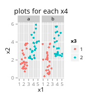
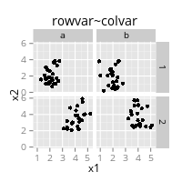
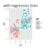
set.seed(1)
x1 <- c(rnorm(500,mean=2,sd=0.5),rnorm(500,mean=4,sd=0.5))
x2 <- c(runif(500,min=0,max=4),runif(500,min=2,max=6))
x3 <- factor(rep(1:2,each=500))
x4 <- rep(c("a","b"),500)
df <- data.frame(x1,x2,x3,x4)

par(mfrow=c(1,2)): number of plots (row=1,col=2)
boxplot(x1,x2,col=3:4) : box-and-whisker plot
boxplot(x1~x3,data=df,col="green"): box-and-whisker plots (with respect to x3)
hist(x1,col="green") : histogram
barplot(table(sequence(1:10)),col="lightblue") : barplot.
plot(1:10,1/(1:10),type="l",col="green",main="type l") : line graph
plot(1:10,1/(1:10),type="b",col="green",main="type b") : both (points and lines)
plot(1:10,1/(1:10),type="b",col="green",main="type c") : both without points
plot(1:10,1/(1:10),type="o",col="green",main="type o") : both (overlapped)
plot(1:10,1/(1:10),type="h",col="green",main="type o") : histogram like vertical lines.
plot(x1,x2,col=x3,pch=20,xlab="xlab",ylab="ylab",xlim=c(0,7),ylim=c(0,7)) : scatterplot of (x1,x2)
- pch=20 : Plot Character
- col=x3 : 1=black, 2=red, 3=green, 4=blue, 5=light blue, 6=pink, ...
- xlab="", ylab="" : labels
- xlim=c(0,7), ylim=c(0,7): drawing region
- For more options.
abline(h=3,lwd=2) :
abline(v=4,col="blue") :
abline(a=2,b=1,col="gren") :
fit.lm <- lm(x2~x1); abline(fit.lm) add a regression line.
lines(vecx,vecy) : draw a segment (connecting points with segments)
points(vecx,vecy,col="lightblue"): add points
title("Scatterplot")
text(vecx,vecy,vecstr) : add text labels vecstr at (vecx,vecy)
axis(1,at=c(0,1440,2880),lab=c("Thu","Fri","Sat")): adding axis ticks/labels. Use xaxt="n" in a plot command.
legend("bottomright",legend=c("one","two"),col=1:2,pch=20)
smoothScatter(rnorm(10000),rnorm(10000)) scatterplot for large number of observations.
pairs(df): scatterplots of all pairs of variables

Color (not finished...)

colors() : the vector of colour names
heat.colors(), topo.colors()
library(colorspace) :
- segments(x0,y0,x1,y=2)
- contour(x,y,f)
- image(x,y,f)
- persp(x,y,f)
library(grDevices) : colorRamp and colorRampPalette. See Color Packages in R Plots.
- colorRamp() : the parameterized segment between given two colors in RGB
- seg <- colorRamp(c("red"),c("blue"))
- seg(0) = [[255,0,0]] (red)
- seg(0.5) = [[127.5,0,127.5]]
- seg(1) = [[0,0,255]] (blue)
- seg(c(0,0.5,1)): gives a table.
- colorRampPalette: Similar to colorRamp, but this gives #ffffff (hex) form
library(RColorBrewer) : three types of palettes: Sequential (low->high), Diverging (neg->0->pos), Qualitative (cats)
cols <- brewer.pal(n=3,name="BuGn"): "#E5F5F9" "#99D8C9" "#2CA25F".

ggplot2

Quick-R: ggplot2 Graphs,

qplot (Quick Plot)

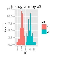
qplot(x1,x2,data=df,color=x3,facets=.~x4,main="plots for each x4")
qplot(x1,x2,data=df,facets=x3~x4,main="rowvar~colvar")
qplot(x1,x2,data=df,color=x3,geom=c("point","smooth"),method="lm",main="with regression lines")
qplot(x1,geom="histogram")

one facet two facets regression

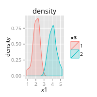
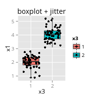
qplot(x1,data=df,fill=x3,binwidth=0.2,main="histogram by x3")
qplot(x1,data=df,color=x3,fill=x3,alpha=I(.2),geom="density",main="density")
qplot(x3,x1,data=df,geom=c("boxplot","jitter"),fill=x3, main="boxplot + jitter")

Histogram Density Boxplot

ggplot2

Official documentation. Plotting distributions (ggplot2)
The followings produces the same graphs as ones which qplot() creates.
- ggplot(df,aes(x1,x2))+geom_point(aes(color=x3))+facet_grid(~x4)+labs(title="plots for each x4")
- ggplot(df,aes(x1,x2))+geom_point()+facet_grid(x3~x4)+labs(title="rowvar~colvar")
- ggplot(df,aes(x1,x2,color=x3))+geom_point()+geom_smooth(method="lm")+labs(title="with regression lines")
- ggplot(df,aes(x1,color=x3,fill=x3))+geom_histogram(binwidth=0.2)+labs(title="histogram by x3")
- ggplot(df,aes(x1,color=x3,fill=x3))+geom_density(alpha=I(0.2))+labs(title="density")
- ggplot(df,aes(x3,x1))+geom_boxplot(aes(fill=x3))+geom_jitter()+labs(title="boxplot + jitter")
drawing steps
1. ggplot(): a data frame (no layer for drawing are created.)
2. geoms_point(), etc. : geometric objects like points, lines, shapes.
3. aes(color=, size=, shape=, alpha=, fill=): aesthetic mappings
4. facet_grid(), facet_wrap() : facets for conditional plots.
5. stats: statistical transformations like binning, quantiles, smoothing.
6. scales: what scale an aesthetic map uses (example: male=red, female=blue)
7. coordinate system: what is it?
geom_point(aes(color=x3)) works but geom_point(color=x3) does not work, unless "x3" consists of colour names.
fill=red, color=blue : background-color: red; border-color:blue;
We can draw something about a different data, by geom_xxxx(data=df2).
geom_smooth(method="lm") : add smooth conditional mean.
geom_histogram(position="dodge",binwidth=2000) : position="stack" is default
geom_hline(yintersept=3): add a line $y=3$.
geom_bar(stat="identity") (Don't use stat="bin")
facet_grid(x3~x4), facet_wrap(x3~x4,nrow=2,ncol=3): add facets (very similar)
theme_gray(): the default theme
theme_bw(base_family="Open Sans",base_size=10): a theme with a white background
labs(title="TITLE",x="x Labal",y="y Labal")
coord_flip() : exchanging the coordinates y ⇆ x
ylim(-3,3), coord_cartesian(ylim=c(-3,3)) : restrict the drawing range to -3≤y≤3
coord_polar(): Polar coordinates
coord_map() : Map projections

scales

Use it together with ggplot(). See RStudio's cheatscheet.
scale_y_continuous(label=comma) : 1000 → 1,000

caret

References: caret, Building Predictive Models in R Using the caret Package (by Max Kuhn)

Resampling

Validation set

inTrain <- createDataPartition(y=df$col1, p=0.75, list=F)
training <- df[inTrain,] ## data frame for training
testing <- df[-inTrain,] ## data frame for testing

The first function createDataPartition(y,p=0.75,list=F) create a boolean vector (so that values of y are uniformly distributed).

The following functions produces a list of training and validation sets.

createFolds(y,k=10,list=T,returnTrain=T): k-fold CV (list of training data sets)
createFolds(y,k=10,list=T,returnTrain=F): k-fold CV (list of test data sets)
createResample(y,times=10,list=T): bootstrap
createTimeSlices(y,initialWindow=20,horizon=10): creates CV sample for time series data. (initialWindow=continued training data, horizon=next testing data)

trainControl

trainControl is used to do resampling automatically when fitting a model.

fitCtrl <- trainControl(method="cv",number=5) ## 5-fold CV

method='boot' : bootstrapping
method='boot632' : bootstrapping with adjustment
method='cv' : cross validation
method='repeatedcv' : repeated cross validation
method='LOOCV' : leave one out cross validation

Preprocessing

General methods for feature engineering are available (Pre-Processing). Before using following functions, we should care about non-numeric columns.

nzv <- nearZeroVar(df,saveMetrics=TRUE) ## vector of columns with small change
df <- df[,-nzv]                         ## remove these columns

nearZeroVar() finds columns which hardly ever changes. Unlike the name, this function do not see variances of predictors.

Correlation

cor(df) gives the matrix of correlations of predictors. Use the package corrplot to look at the heat map of the matrix. (Manual,Vignette)

library(corrplot)
corrplot.mixed(cor(df)) ## heatmap + correlation (as real values)

A standard heatmap can be created by corrplot(cor(df),method="color").

findCorrelation() is used to remove highly correlated columns.

hCor <- findCorrelation(cor(df),cutoff=0.75) ## highly correlated columns
df <- df[,-hCor] ## remove these columns

Standardisation with preProcess

preProc <- preProcess(df.train,method=c("center","scale"))
df.train.n <- predict(preProc,df.train) ## standardising df.train w.r.t. preProc.
df.test.n <- predict(preProc,df.test)   ## standardising df.test w.r.t. preProc.

preProcess() creates an object with normalisation data (i.e. means and standard deviations). To normalise data, use predict() function as above.

The factor variables are safely ignored by preProcess().
preProc$mean : same as apply(df.train,2,mean)
preProc$std : same as apply(df.train,2,sd)

PCA with preProcess()

preProc <- preProcess(df,method="pca",pcaComp=ncol(df)) ## PCA
Xpc <- predict(preProc,df) ## feature matrix w.r.t. principal components

With method='pca' the original feature matrix is automatically normalised unlike prcomp(). (See below.) Therefore $\sum_{i=1}^p \mathrm{Var}(Z_i) = p$ holds. Here $Z_i$ is the i-th principal component.

The factor variables are safely ignored by preProcess()
pcaComp : the number of principal components we use.
preProc$rotation : the matrix $R$ such that $X_{pc} = X_n R$. Here $X_n$ is the normalised feature matrix.

PCA without caret

prComp <- prcomp(df) ## compute the principal components
Xpc <- prComp$x      ## feature matrix with respect to principal components

prComp contains the result of PCA. This function makes a given matrix centered, but to normalise with standard deviation, then scale=TRUE is needed.

prComp$x : the feature matrix after PCA.
prComp$center : same as apply(X,2,mean)
prComp$sdev : standard deviation of principal components
prComp$scale : same as apply(X,2,sd) if the option scale=TRUE is used.
prComp$rotation : the matrix $R$ such that $X_{pc} = X_c R$. Here $X_c$ is the centered feature matrix.

Namely the feature matrix Xpc with respect to PCA can also be calculated.

Xc <- X - matrix(1,nrow=nrow(X),ncol=ncol(X)) %*% diag(prComp$center)   ## centerise
Xn <- Xc * (matrix(1,nrow=nrow(X),ncol=ncol(X)) %*% diag(1/prComp$scale)) ## rescale
Xpc <- Xc %*% prComp$rotation

The same formula can be used to compute a feature matrix of the validation/test set with respect principal components.

Fit a model

The train() function fits a model:

fit.glm <- train(y~.,data=df,method='glm',trControl=fitCtrl,tuneGrid=fitGrid)
yhat <- predict(fit.glm,newdata=df.test)

This function executes also validation (with bootstrapping). Therefore it is better to specify a validation method explicitly.

train() is a wrapper function of functions producing predictive models.
The method option specifies a statistic model (model list).
The trControl option specifies a validation method and takes output of trainControl(). (See above.)
We can manually specify values of tuning parameter to try, using the tuneGrid option.
fit.glm$finalModel
fit.glm$results data.frame of the grid search
- method="gam" : Generalised Additive Model using Splines
- method="gbm" : Stochastic Gradient Boosting. Don't forget verbose=F
- method="lda" : Linear Discriminant Analysis
- method="nb" : Naive Bayes
- method="rf" : Random Forest
- method="rpart" : CART (Decision tree)

How to show the results (This section is going to be removed.)

print(fit.glm) or just fit.glm : overview of the result.
summary(fit.glm) : some details
names(fit.glm) : Do not forget to check what kind of information is available.
sqrt(mean((predict(fit.glm)-training$y)^2): root-mean-square error (RMSE) on training set sqrt(mean((prediction-training$y)^2): RMSE on testing set
confusionMatrix(predict(fit.glm,newdata=),testing$col1): check the accuracy.
plot.enet(model.lasso$finalModel,xvar="penalty",use.color=T) : graph of the coefficients in penalty parameter
featurePlot(x=training[,vec],y=training$col,plot="pairs"): lattice graphs
- box, strip, density, pairs, ellipse : plot for classification
- pairs, scatter: plot for regression
library(partykit); plot(fit); text(fit); plot(as.party(fit),tp_args=T) : for decision tree.
order(...,decreasing=F):

Binary Classification

	Actual negative	Actual positive
predicted negative	True Negative	False Negative (Type 2 error)
predicted positive	False Positive (Type 1 error)	True Positive

Specificity := True Negative$/$Actual Negative
FP rate := False Positive$/$Actual Negative (1-specificity)
Recall: R := True Positive$/$Actual Positive (a.k.a. sensitivity or TP rate)
Precision: P := True Positive$/$Predicted Positive (a.k.a. Pos. Pred. Value.)
F₁-score := 2PR/(P+R)

For a vector of labels (0 or 1) and a vector of probabilities of $Y=1$, the following function creates a data frame of accuracies, FP rates, TP rates, precisions and F1 scores by thresholds.

accuracy.df <- function(label,proba,thresholds=seq(0,1,length=100)) {
    accuracy.df <- data.frame()
    for (t in thresholds) {
        prediction <- ifelse(proba > t, 1 ,0)
        TN <- sum(prediction==0 & label==0)
        FN <- sum(prediction==0 & label==1)
        FP <- sum(prediction==1 & label==0)
        TP <- sum(prediction==1 & label==1)
        accuracy <- (TN+TP)/(TN+FN+FP+TP)
        FPrate <- FP/(TN+FP)  ## x for ROC (1-specificity)
        TPrate <- TP/(TP+FN)  ## y for ROC (recall)
        precision <- TP/(FP+TP)
        F1score <- 2*TPrate*precision/(TPrate+precision)
        accuracy.df <- rbind(accuracy.df,
                             data.frame(t=t,
                                        accuracy=accuracy,
                                        FPrate=FPrate,
                                        TPrate=TPrate,
                                        precision=precision,
                                        F1score=F1score))
    }
    return(accuracy.df)
}

The following command draws two graphs of accuracies and F1 scores.

ggplot(df,aes(x=t,y=accuracy,color='accuracy')) + geom_path() + 
    geom_path(data=df,aes(x=t,y=F1score,color='F1score')) + labs(x='threshold',y='')

ROC

Using the data frame produced by the above accuracy.df() function, we can draw something like the ROC (Receiver Operating Characteristic) curve:

ggplot(adh,aes(x=FPrate,y=TPrate))+geom_step() ## NOT a rigorous ROC curve

But there is a package for drawing it: ROCR. (cf. ISLR P. 365.)

library(ROCR) ## contains performance()
rocplot <- function(pred,truth,...){
    predob <- prediction(pred,truth)
    perf <- performance(predob,"tpr","fpr")
    plot(perf,...)
}

Here pred (resp. truth) is a vector containing numerical score (resp. the class label) for each observation.

One way to determine a good threshold is to choose a threshold so that TP rate − FP rate is maximum.

Statistical Modells

Linear Regression with/without penalty term

The standard linear regression can be fitted by the following functions.

fit.glm <- train(y~.,data=df,method='glm') ## with caret 
fit.glm <- glm(y~.,data=df)                ## without caret

Elasticnet (Ridge Regression, Lasso and more)

The elasticnet model is provided by glmnet.

enetGrid <- expand.grid(alpha=c(0,10^(-3:0)),lambda=c(0,10^(-3:0)))
fit.eln <- train(y~.,data=df,method='glmnet',tuneGrid=enetGrid)

The elesticnet penalty is defined by

$$\lambda\left(\frac{1-\alpha}{2}\|\beta\|_2^2 + \alpha\|\beta\|_1^2\right) \qquad (0\leq\alpha\leq 1).$$

This is slightly different from one in ESL (P.73). We take the norms after removing the intecept as usual.

If $\alpha=0$, then it is (half of) the ridge penalty $\lambda\|\beta\|_2^2/2$.
If $\alpha=1$, then it is the lasso penalty $\lambda\|\beta\|_1^2$.
The objective function is defined by RSS/2 + (elasticnet penalty).
Note that glmnet can also be used for classification. An objective function for a classification is given by -log(likelihood) + (elasticnet penalty).
(In a training process, a feature matrix must be automatically rescaled by the default behavior of the function.)

There are a few tipps to use glmnet package without caret.

library(glmnet)
X <- as.matrix(select(df,-y)) ## dplyr::select is used
y <- df$y
ridge.mod <- glmnet(X,y,alpha=0,lambda=2) ## ridge

We have to use a matrix instead of a data frame. y must also be a vector of numbers.
As a default this function standardize the variables. The returned coefficients are on the original scale, but if the variables are in the same unit, then we should turn it of with standardize=FALSE.

The elasticnet package provides similar functions as well and we can use it through caret by method=enet (elasticnet), method=ridge (ridge regression) and method=lasso (lasso).

(Penalised) Logistic Regression

Consider a classification problem with $K$-classes $1, \cdots, K$. In logistic regression [ISLR P.130. ESL P.119] is a mathematical model of form

$$\mathbb P(Y=k|X=x) = \begin{cases} \dfrac{\exp\langle\beta_k,x\rangle}{1+\sum_{l=1}^{k-1}\exp\langle\beta_l,x\rangle} & (k=1,\cdots,K-1) \\ \dfrac{1}{1+\sum_{l=1}^{k-1}\exp\langle\beta_l,x\rangle} & (k=K) \end{cases}$$

We denote by $g_i$ the class to which $x_i$ belongs and we set $x_0 \equiv 1$as in linear regression.

The objective function is defined by $J_\lambda(\beta) = -\ell(\beta) + (\mathrm{penalty})$. Here $\ell(\beta)$ is the log-likelihood function defined by $$\ell(\beta) = \sum_{k=1}^K \sum_{x_i: g_i=k} \log \mathbb P(Y=k|X=x_i;\beta).$$

Elasticnet (glmnet)

We can use glmnet for logistic regression with elastic penalty. See above. (Note that the elasticnet package is only for regression.)

stepPlr

When we fit a logistic regression model with $L_2$ penalty $\lambda\|\beta\|^2$, we can also use the stepPlr package.

plrGrid <- expand.grid(lambda=c(0,10^(-3:0)),cp='bic')
fit.plr <- train(y~.,data=df,method='plr',tuneGrid=plrGrid)

There are some remarks to use the plr function ofstepPlr directly.

library(stepPlr)
X <- df[3:4]                         ## X must contains only features used.
y <- ifelse(df$default=='Yes', 1, 0) ## y must a vector of 0 and 1.
fit.plr <- plr(y=y,x=X,lambda=1)

Note that the target variable must take only 0 and 1, so basically this can be used only for a binary classification. (But caret fit a multi-class classification with stepPlr. I do not know exactly what caret does.)

fit.plr$coefficients : estimated parameters (incl. the intercept)
fit.plr$covariance : covariance matrix
fit.plr$deviance : (residual) deviance of the fitted model, i.e. $-2\ell(\hat\beta)$.
fit.plr$cp complexity parameter ("aic" => 2, "bic"=> $\log(n)$ (default))
fit.plr$score : deviance + cp*df. Here df is the degree of freedom.
fit.plr$fitted.values : fitted probabilities.
fit.plr$linear.predictors : $X\beta$.

Use predict.plr() to predict the probabilities.

pred.test.proba <- predict.plr(fit.plr,newx=Xtest,type="response") ## probabilities
pred.test.class <- predict.plr(fit.plr,newx=Xtest,type="class")    ## classes (0 or 1)

multinom in nnet

This is a logistic regression as a special case of a feed-forward neural network. This function is provided by nnet.

mltGrid <- expand.grid(decay=c(0,10^(-3:0)),cp='bic')
fit.mlt <- train(y~.,data=df,method='multinom',tuneGrid=mltGrid)

Without caret:

library(nnet)
fit.mm <- multinom(y~.,df,decay=0,entropy=TRUE)

decay=0 : the coefficient of the penalty term (i.e. $\lambda$).
fit.mm$AIC : the AIC

Linear/Quadratic Descriminant Analysis (LDA/QDA)

library(MASS)
fit.lda <- lda(y~.,data=df) ## qda(y~.,data=df) for QDA 
pred <- predict(fit.lda,df)

ISLR P. 138. ESL P. 106. In caret method="lda" / method="qda".
A target variable $Y := 1, \cdots, K$ (classification)
$\pi_k := \mathbb P(Y=k)$ : the prior probability of the $k$-th class
$f_k(x) := \mathbb P(X=x|Y=k)$ : the PDF of $X$ for the $k$-th class

$$\mathbb P(Y=k|X=x) = \dfrac{\pi_k f_k(x)}{\sum_{l=1}^K \pi_l f_l(x)}\quad$$

LDA : We assume $X \sim \mathcal N(\mu_k, \Sigma)$. (The covariance matrix is common.)
QDA : Wa assume $X \sim \mathcal N(\mu_k, \Sigma_k)$
fit.lda$prior : estimated prior probability i.e. $\hat\pi_1$, $\hat\pi_2$, ...
fit.lda$means : average of variables by group, i.e. $\hat\mu_1$, $\hat\mu_2$, ...
fit.lda$scaling : coefficients of linear/quadratic discriminant.
plot(fit.lda) : "normalised" histogram of the LDA decision rule by group. (Only for LDA.)
pred$class : LDA's prediction about the class. (matrix)
pred$posterior: probabilities
pred$x : the linear descriminants (Only for LDA.)

K-Nearest Neibours (KNN)

library(class)
set.seed(1)
knn.pred <- knn(train=X,test=Xtest,cl=y,k=1)

A random value is used when we have ties.
We should be care about the scale of each variable because of the distances.
knn.pred is the vector of the predicted classes.

Support Vector Machine

ISLR P.337, ESL P.417. The explanation in this section is based on the course "Machine Learning by Prof. Ng" (Lecture Notes).

We describe only the case of a binary classification: $y=0,1$. There are two basic ideas:

We allow a margin when we determine a decision boundary.
We create new $n$ predictors with a kernel $K$ to obtain a non-linear decision boundary.

A kernel is a function describing the similarity of two vectors and the following kernels are often used.

linear kernel : $K(u,v) := \langle u,v \rangle$
polynomial kernel : $K(u,v) := (c_0+\gamma\langle u,v \rangle)^d$
radial kernel : $K(u,v) := \exp\bigl(-\gamma\|u-v\|^2\bigr)$
sigmoid kernel : $K(u,v) := \mathrm{tanh}(c_0+\gamma\langle u,v \rangle)$

For an observation $x^*$ a new "feature vector" is defined by $K(x^*) := (1,K(x^*,x^1),\cdots,K(x^*,x^n))$.

The optimisation problem is $$\min_\theta C \sum_{i=1}^n \Bigl( y^i \mathrm{cost}_1 (K(x^i)\theta) + (1-y^i)\mathrm{cost}_0 (K(x^i)\theta) \Bigr) + \frac{1}{2}\sum_{i=1}^n \theta_i^2 $$ Here

$\theta = (\theta_0,\cdots,\theta_n)^T$ is a column vector of parameters.
$\mathrm{cost}_0(z) := \max(0,1+z)$ and $\mathrm{cost}_1(z) := \max(0,1-z)$.
$C$ is a positive tuning parameter called "cost". If $C$ is small, then the margin is large.
We use only part of observations to create new features. (Namely the support vectors.) Thus the actual number of features are smaller than $n+1$.

For an observation $x^*$ we predict $y=1$ if $K(x^*)\theta \geq 0$. The function $K\theta$ is called the SVM classifier.

library(e1071)
fit.svm <- svm(y~.,data=df,kernel='radial',gamma=1,cost=1)

The target variable must be a factor, when we deal with a classification.
Specify the kernel function with the kernel option. ("radial" is the default value.)
Tuning parameters: cost=$C$, gamma=$\gamma$, coef0=$c_0$, degree=$d$
Use the scale option is a logical vector indicating the predictors to be scaled.
The caret package uses e1071 for the linear kernel and kernlab for other kernels. Because of this the options of tuning parameters are different.

The object of class "svm" contains

fit.svm$SV : (scalled) support vectors
fit.svm$index : the indexes of the support vectors
fit.svm$coefs : the corresponding coefficients times training labels
fit.rho : the negative intercept

plot(fit.svm,df) draws a 2d scatter plot with the decision boundary.

Decision Tree

(not yet)

Random Forest

ISLR P. 329. ELS P.587. Practical Predictive Analytics: Models and Methods (Week 2)

The random forest uses lots of decision trees of parts of data which are randomly chosen. Using trees, we make a prediction by majoirty vote (classification) or average among the trees. A rough algorithm is following.

Draw a bootstrap sample of size $n$ and select $m$ predictors at random ($m < p$).
Create a decision tree of the bootstrap sample with selected predictors.
Repeat 1 and 2 to get trees $T_1,\cdots,T_B$.
Take a vote (for classification) or the average (regression).

The randomForest package provides the random forest algorithm.

library(randomForest)
set.seed(1)
fit.rf <- randomForest(medv~.,data=df.train,mtry=13,importance=T)

mtry : number of predictors randomly selected. The default value is $\sqrt{p}$ for classification and $\sqrt{p/3}$ for regression. If large number of predictors are correlated, we should choose a small number.
ntree : number of trees to grow

An object of the class "randomForest" contains:

fit.rf$predicted: predicted values for training set
For classification
- fit.rf$confusion : the confusion matrix
- fit.rf$err.rate : the (OOB) error rate for all trees up to i-th.
- fit.rf$votes : the votes of trees in rate.
For regression
- fit.rf$mse : vector of MSE of each tree.
fit.rf$importance : as follows.

The variable importance is based on the following idea: scramble the values of a variable. If the accuracy of your tree does not change, then the variable is not very important. fit.rf$importance is a data frame whose columns are classes, MeanDecreaseAccuracy and MeanDecreaseGini (for classification) or IncMSE and IncNodePurity (for regression).

nnet

The package nnet (Manual) provides a feed-forward neural network model with one hidden layer.

library(nnet)
xor.df <- data.frame(x0=c(0,0,1,1),x1=c(0,1,0,1),y=c(0,1,1,0))
xor.fit <- nnet(y~.,xor.df,size=2,entropy=TRUE)
predict(xor.fit,type='class')

The above code is for a feed-forward neural network model for XOR. The BFGS method is used for optimization.

size : the number of hidden units in the hidden layer.
entropy=FALSE : the objective function. The default is the squared error. If entropy=TRUE, the cross-entropy is used.
linout=FALSE : the activation function or the output unit. The default is the logistic function. If linout=TRUE then the activation function is linear.
decay=0 : the weight decay (the coefficient of the penalty term).

summary(xor.fit) shows the trained weights

summary(xor.fit)
## a 2-2-1 network with 9 weights
## options were - entropy fitting 
##  b->h1 i1->h1 i2->h1 
## -29.19 -33.45  39.81 
##  b->h2 i1->h2 i2->h2 
##   8.54 -22.99  19.75 
##   b->o  h1->o  h2->o 
##  12.95  51.84 -30.66

neuralnet

manual

MXNet

doc

Parameter tuning

The tune() function tunes parameters with 10-fold CV using a grid search over a specified paramter ranges.

library(e1071)
set.seed(1)
tune.out <- tune(svm,y~.,data=df,kernel="radial",ranges=list(cost=c(0.1,1,10,100,1000),gamma=c(0.5,1,2,3,4)))

Options:

method : the function to be turned. (method=svm in the above example.)
ranges : a named list of parameter vectors.
tunecontrol : for a turning method. This accepts an object created by tune.control().
- tunecontrol=tune.control(sampling="cross",cross=10) : 10-fold CV
- tunecontrol=tune.control(sampling="bootstrap") : bootstrapping
- tunecontrol=tune.control(sampling="fix") : single split into training/validation set

An "tune" object contains:

tune.out$best.parameters : the best parameters
tune.out$best.performance : the best achieved performance (error rate or MSE).
tune.out$train.ind : the indexes of observations in the training set of each CV
tune.out$sampling : turning method (e.g. "10-fold cross validation")
tune.out$performances : the data frame of performances for each turning parameter.
tune.out$best.model : the model obtained with the best parameters. For example we can use it for predict().

plot(tune.out) gives the graph of performance. transform.x=log10 might be help.

Examples of the ranges option

Support Vector Machine

param.grid <- list(
    cost   = 0.01*(2^(1:10))       ## 0.02, 0.04, 0.08, ..., 10.24
    gamma  = 10^(1:5-3)            ## 1e-02, 1e-01, 1e+00, 1e+01, 1e+02
    kernel = c("radial","sigmoid")
)

Random Forest

param.grid <- list(
    mtry = 2:ceiling(sqrt(ncol(df))), ## replace "ncol(df)" with a suitable number
    ntree = seq(100,500,length=5)     ## 100, 200, 300, 400, 500
)

K-Nearest Neighbourhood: use tune.knn():
```
tune.knn <- tune.knn(X,y,k=1:10)
```
nnet (penalised logistic regression)
```
grid.param <- list(decay=10^(1:7-5))
```

K-means clustering

Example. See also ISLR §10.5.1. ykmeans: K-means using a target variable.
km.out <- kmeans(df,centers=3,nstart=20) : K-Means Clustering
- nstart=20 : how many random sets should be chosen. (It should be large.)
- km.out$cluster : integer vector of results
- km.out$tot.withinss : total within-cluster sum of squares
hc.out <- hclust(dist(x),method="complete") :
- dist() : compute the matrix of (euclidean) distances b/w observations
- method : linkage (complete, average, single, etc.)
- plot(hc.out) : show the result
cutree(hc.out,k=2) : reduce the number of clusters

leaps

fit.full <- regsubsets(y~.,data=df,nvmax=10) : Regression subset selection. Details.
- nvmax : maximum size of subsets to examine
fit.smry <- summary(fit.full)
- fit.smry$cp : Mallows' Cp
- fit.smry$adjr2 : Adjusted r-squared
plot(fit.full,scale="Cp") : visualisation of the summary

fmsb (for raderchart)

The package for a rader chart (a.k.a. spider plot). Manual.
radarchart(df,seg=5,plty=5,plwd=4,pcol=rainbow(5)).
A radar chart with ggplot2.

Miscellaneous

ls() : vector of names of defined variables
rm(list=ls()) : delete the defined variables
with(df, function(...)) : in ... we can use names(df)

mlR

Tutorial

Task

manual

cost-sensitive classification

Feature Selection

manual

Learner

no learner class for cost-sensitive classification => classification

List of integrated learners

Classification:
Regression:

lrn$par.vals current setting of meta parameters lrn$par.set list of meta parameters

Train and Prediction

Performance Measure

performance()

performance(yhat,measure=acc) (Note that no quotation for acc is needed.) measure=list(acc,mmce) works.

if you measure your clustering analysis you will need

list of metrics

mmce (mean misclassification error)
acc (accuracy)
mse (mean of squared errors)
mae (mean of absolute errors)
medse (median of squared errors)
dunn (Dunn index) : for clustering
mcp (missclassification penalty)

ROC curve?

Documentation

HTML and PDF

R Markdown (including manual and links). An template for an HTML document is following.

---
title: "TITLE"
author: "NAME"
date: "01.01.2016"
output:
  html_document:
    theme: flatly
    toc: true
---

The white space for the nesting is important. The toc option is for an table of contents.
When we need a Markdown file (and images), put keep_md: true in the html_document option.

To compile an Rmd file, use the following shell command.

user$ R --quiet -e "rmarkdown::render('test.Rmd')"

To obtain a PDF file instead of an HTML file, use the following. (No need to change the header.)

user$ R --quiet -e "rmarkdown::render('test.Rmd','pdf_document')"

Embedding Codes

```{r}
library(ggplot2)
ggplot(iris,aes(x=Petal.Length,y=Petal.Width,color=Species))+geom_point()
```

option	execute	code chunk	result
`eval=FALSE`	no	shown	no
`results="hide"`	yes	shown	hidden
`echo=FALSE`	yes	hidden	shown

warning=FALSE
message=FALSE

ioslides

There are a few ways (including Slidify) to produce slides with R Markdown. (Comparison.) Here we use ioslides (Manual for R markdown) to create slides.

An easy example of YAML header is following. (We can create slides in a similar way to an PDF file as above, but we should create a different file because of the syntax for slides.)

---
title: "TITLE"
author: "NAME"
date: "01.01.2016"
output:
  ioslides_presentation:
    widescreen: true
    smaller: true
---

The options fig_height: 5 and fig_width: 7 in output change the size of the images.

After opening the created HTML file, several shortcut keys are available: f for the fullscreen mode and w for the widescreen mode.

MathJax

We can use MathJax to describe mathematical formula. This means that the slides require Internet connection.

If you can not expect Internet connection, then convert the slides into a single PDF file. (For the conversion see below.)

If you can use the own PC, you can also use a local copy of MathJax.

  ioslides_presentation:
    mathjax: "http://localhost/mathjax/MathJax.js?config=TeX-AMS-MML_HTMLorMML"

In any case, you should prepare a PDF file of slides!

Markup Rules

An subsection ## is a slide.
We need 4 spaces to nest a list.
For incremental bullets, put > before hyphens.
How to create a table.

Slides in a PDF file

We use the same command as HTML to produce the slides. The slides are contained in a single HTML file. To produce a PDF file we should use google-chrome with the following printing settings.

Layout: Querformat
Ränder: Keine
mit Hintergrundgrafiken

Share this page on