In the last entry of this series, I introduced useful Perl modules for data mining. In this entry we finally do data mining with Perl.

Arrow::DataFrame

I am writing a Perl module Arrow::DataFrame for data-mining. This is a degenerated version of a data frame of R and methods are very similar to corresponding functions of R.

The module is not finished yet. (For example no merge() method.) But most of fundamental methods for manipulation (equivalent to dplyr of R) are already available. I would like you to read the manual for more details.

PDL

We use PDL for numerical computation. (However I said in the last entry that I did not use it for a while.) PDL is something like "numpy" in Perl. Namely PDL allows us to solve many problems in a short time.

• PDL official website provides nice tutorials. (Or $ perldoc PDL::Tutorial.)
• RFC: Getting Started with PDL (the Perl Data Language)
• David Mertens Introduction to the Perl Data Language (youtube video)
• RFC: PDL Cheat Sheet

Linear Regression with/without penalty

A very brief review of linear regression

The main topic of this entry is linear regression and a role of a penalty term. Let us introduce breifly notation for it. Assume that we have $n$ observations and $p$ predictors (features). We denote by $Y^i$ a target variable. A linear model is

$$Y^i = \beta_0 + \beta_1 x^i_1 + \cdots + \beta_p x^i_p + \varepsilon^i \quad(i=1,\cdots,n)$$

with (regression) parameters $\beta_0, \cdots, \beta_p$, where $\varepsilon^1,\cdots,\varepsilon^n$ are i.i.d. random variables with $\varepsilon^1 \sim \mathcal N(0,\sigma^2)$ for some positive $\sigma$. We define a design matrix $X$ by

$$X := \begin{pmatrix} 1 & x^1_1 & \cdots & x^1_p \\ \vdots & \vdots & \ddots & \vdots \\1 & x^n_1 & \cdots & x^n_p \end{pmatrix}.$$

Then we can write the linear model in a simple form: $Y = X\beta + \varepsilon$.

Given observations $Y = y = (y^1,\cdots,y^n)^T$, we employ the squared error $\| y - X\beta \|^2$ for our optimisation objective. Regarding $X$ as a linear map $\mathbb R^p \to \mathbb R^n$, the squared error is minimum iff $P_W y = X\beta$. Here $W$ is the image of $X$ and $P_W$ is the orthogonal projection to $W$. Therefore there is a unique parameter vector $\beta$ up to $\ker X$ which minimizes the squared error.

Assuming that $X$ is injective, we have a well-defined linear function $\hat\beta:\mathbb R^n \to \mathbb R^p$ which satisfies $P_W y = X\hat\beta(y)$. We have an explicit formula of $\hat\beta$:

$$\hat\beta(Y) = (X^TX)^{-1}X^TY.$$

We note that the symmetric matrix $X^TX$ is invertible if $X$ is injective. This is an easy conclusion of the fact that $\|X^TXv\|^2=0$ implies $v=0$. A way to find the above formula is to solve $\mathrm{grad}\ \|y-X\beta\|^2 = 0$. (Note that $\beta$ is the only variable.) Another way is to observe that $P_W = X(X^TX)^{-1}X^T$. It might be difficult to find it in a heuristic way, but it is easy to see that the RHS is the orthogonal projection to $W$.

The bias-variance trade-off

We are assuming that $y=f(x) + \varepsilon$ holds as a "real" relation and we can estimate the parameter $\beta$ as a linear map $\hat\beta$. So we have an predictive model $\hat y = \hat f (x) := \langle x, \hat\beta \rangle$. Given a new observation $(x^0,y^0)$, we have the bias-variance decomposition [ISLR, Section 2.2.2].

$$\mathbb E \bigl( (y^0 - \hat f (x^0))^2 \bigr) = \mathsf{Var}(\hat f(x^0))+\mathsf{Bias}(\hat f(x^0))^2 + \mathsf{Var}(\varepsilon).$$

The LHS is the expected test MSE. This is what we want to make small actually.

The variance, the first term of the RHS, describes how much change $\hat f$ if we use other training data. Therefore the smaller the variance is, the more stable the estimation is with respect to training data. We may say: the smaller the variance is, the more we can trust the predictive model.

The bias, the second term of the RHS, describes the difference between the "real" model and the expected value of our model. Thus the smaller bias is, the more accurate the predictive model is.

The irreducible error, the last term $\mathsf{Var}(\varepsilon)$, is beyond our control.

A good predictive model should have low variance and low bias (squared) at the same time. The bias-variance trade-off refers the phenomenon that the variance will increase if we make the bias small, and the bias will increase if we make the variance small. (A good example can be found in ESL Section 2.9.)

The role of the penalty term

Now we assume that $y = \langle x,\beta \rangle + \varepsilon$. Since $\hat\beta \sim \mathcal N(\beta,\sigma^2(X^TX)^{-1})$, we have

$$\mathsf{Var}(\hat f(x)) = \sigma^2 x^T (X^TX)^{-1} x, \quad \mathsf{Bias}(\hat f(x)) = f(x) - \mathbb E(\hat f(x)) = 0.$$

Thus what we can only do is: to make the variance smaller by allowing the bias to increase. The penalty term is exactly for it. Our new optimisation objective is given by

$$ J_\lambda(\beta) = \| y - X\beta \|^2 + \lambda\| \beta' \|^2 $$

for $\lambda \geq 0$. Here $\beta' = (\beta_1,\cdots,\beta_p)$. If $\lambda = 0$, then $J_\lambda(\beta)$ is nothing but the squared error. Thus if $\lambda$ is small, then $\hat\beta$, which minimizes $J_\lambda(\beta)$, is closed to $P_W y$. If $\lambda$ is large, then $\beta'$ is close to the origin. This observation implies intuitively that the bias of our new predictive model $\hat f (x) = \langle x, \hat\beta \rangle$ will increase and the variance will be small because of small $\|\beta'\|$.

Remark. Our discussion about the variance and the bias is different from one in ISLR. This is because we assume an explicit formula for the real relation $y=f(x)$, while we do not in ISLR. We hardly ever know the explicit formula, therefore we can not compute the bias in practice.

How the variance decreases

First we note that we have an explicit formula of $\hat\beta$:

$$\hat\beta(y) = (X^TX + \lambda I'_p)^{-1}X^Ty.$$

Here $I'_p$ is the diagonal matrix $\mathsf{diag}(0,1,\cdots,1)$ of size $p+1$. The solution can be obtain by solving the equation $\mathsf{grad}\!\ J_\lambda(\beta) = 0$.

Now we assume that our design matrix $X$ is centred (except the first column). Namely the sample mean of each column is 0. Then the estimated intercept $\hat\beta_0$ is given by the sample mean of $y = (y^1,\cdots,y^n)$ and $\beta'$ is given by

$$\hat\beta'(y) = (X^TX + \lambda I_p)^{-1}X^Ty.$$

Here $X$ is NOT the design matrix, but the $n \times p$ matrix $X = (x^i_j)_{i,j}$ ($i = 1,\cdots,n, j = 1,\cdots,p$). (See also ESL Section 3.4.1.) This formula follows from the formula of $\hat\beta(y)$:

$$\hat\beta(y) = \begin{pmatrix} n & 0 \\ 0 & X^TX + \lambda I_p \end{pmatrix}^{-1} \begin{pmatrix} 1 \cdots 1 \\ X^T\end{pmatrix} y.$$

Now $\hat\beta_0$ is independent of $\lambda$ and $\hat\beta' \sim \mathcal N(C\beta',\sigma^2 LL^T)$, where $C$ and $L$ are determined by the following calculation.

$$\hat\beta'(Y) = (X^TX+\lambda I_p)^{-1} X^T ( X\beta' + \varepsilon ) = C \beta' + \sigma L \frac{\varepsilon}{\sigma} $$

Since $X^TX$ is symmetric, it is diagonalisable with an orthogonal matrix $V \in O(p)$. Thus we have $V^{-1}(X^TX)V = \mathsf{diag}(d_1,\cdots,d_p) =: D$. Here the eigenvalues $d_j$ ($j = 1,\cdots,p$) of $X^TX$ are non-negative, and all positive if $X$ is injective. An easy calculation shows that the matrix $LL^T$ is also diagonalisable with $V$ and the eigenvalues are

$$\frac{d_1}{(d_1+\lambda)^2},\ \cdots,\ \frac{d_p}{(d_p+\lambda)^2}.$$

The larger $\lambda$ is, the smaller the eigenvalues of the covariance matrix of $\beta'$ are. (If some of $d_i$ are close to 0, i.e. some columns of $X$ are "nearly" linear dependent, then the effect of $\lambda$ will be very large.) These formulas show how the variance will decrease if $\lambda$ increases.

A side effect of the penalty term

It is well-known that we can apply the ridge regression (linear regression with penalty term) even though $X$ is not injective.

$$X^TX + \lambda I_p = V^{-1} \mathsf{diag} (d_1+\lambda,\cdots,d_p+\lambda) V$$

Therefore the LHS is invertible whenever $\lambda$ > $0$.

Time to experiment

Data and scripts

We use prostate.data which can be obtained at the ESL website. The data are used in ESL Section 3.4 to explain the shrinkage methods.

Our scripts can be found my Bitbucket repository. We execute ridge.pl and we assume the following directory structure.

.
├── Arrow
│   ├── DataFrame.pm
│   ├── GroupBy.pm
│   ├── LinearRegression.pm
│   └── Model.pm
├── prostate.data
└── ridge.pl

I also provide a IPython notebook ridge.ipynb with a few comments. (An HTML version is available.)

The Perl script in detalis

We read part of our perl script in details.

The following modules are used. The first one is to read the data and manipulate it. The second one is to construct a predictive model (linear/ridge regression). The third one is for numerical computation.

use Arrow::DataFrame;
use Arrow::Model qw(LinearRegression);
use PDL;

First we read the data. The first column is the index without name, so give it a name, then remove it.

my $df = Arrow::DataFrame->read_csv("prostate.data",{sep_char=>"\t"});
$df->set_name('id',0);    ## give a name to the first column
$df = $df->select('-id'); ## delete the first column

The last column indicates which observation is in training data. We use the column to divide the data into training data and test data. The target variable is "lpsa".

my $df_train = $df->filter_th(sub { $_[0]{train} eq 'T' })->select('-train');
my $y_train = $df_train->select('lpsa')->as_pdl;
my $X_train = $df_train->select('-lpsa')->as_pdl;

Next we standardise the data: $X_j \mapsto (X_j - \bar X_j)/\sigma_j$. We do not need to do it to apply linear/ridge regression, but it is very important in practice as we will see later.

my ($p,$n) = dims($X_train); ## $n is the number of observations
my $mu = (1/$n) * ones($n,1) x $X_train; ## means of columns
my $sigma = sqrt((1/($n-1)) * ones($n,1) x ($X_train-$mu)**2 ); ## std of columns
$X_train = ($X_train - $mu) / $sigma;

We prepare the test data. We pick the rows with train == 'F' and remove the column. We also standardize the data in the same way as the training data. (We have to use the same formula.)

my $df_test = $df->filter_th(sub { $_[0]{train} eq 'F' })->select('-train');
my $y_test = $df_test->select('lpsa')->as_pdl;
my $X_test = $df_test->select('-lpsa')->as_pdl;
$X_test = ($X_test - $mu) / $sigma;

A linear model fits the data. The usage of Arrow::Model::LinearRegression is pretty similar to scikit-learn. First we create an instance, then we use the fit()-method to estimate regression parameters, and finally we predict the target variable on the test set.

my $estimator_lr = LinearRegression();      ## model_lr = LinearRegression()
$estimator_lr->fit($X_train,$y_train);      ## model_lr.fit(X_train,y_train)
my $yhat = $estimator_lr->predict($X_test); ## yhat = model_lr.predict(X_test)

After creating a predictive model, we print the scores (RMSE and R^2) of the model on both training data and the test data. The following line computes a matrix $P of eigenvectors and an array $D of eigenvalues. We use only the latter.

my ($P,$D) = eigens($X_train->transpose x $X_train);

After that we compute the RMSE (train and test), the R^2 (R2_train and R2_test), regression parameters (beta1, ..., beta8) and $d_j/(d_j+\lambda)^2$ for each $j$ (d1,...,d8).

my @names = qw(log10(lambda) lambda train test R2_train R2_test);
push(@names, map{ "beta".$_ } 1..$p);
push(@names, map{ "d".$_ } 1..$p);
my $df_ridge = Arrow::DataFrame->new(names=>\@names);

foreach my $lambda (map { 10**(-1 + (3/99)*$_) } 0..99) {
  ## create a predictive model for each $lambda (skipped)
  ## compute the scores, etc. (skipped)
  $df_ridge = $df_ridge->rbind(\@row);
}

We show the best predictive models by looking at RMSE and R^2. These are basically equivalent to each other, so the result are the same.

print "\nSmall RMSE TOP 3\n";
$df_ridge->arrange('test')->select('log10(lambda):R2_test')->head(3);
print "\nR2 score TOP 3\n";
$df_ridge->arrange(['R2_test',desc=>1])->select('log10(lambda):R2_test')->head(3);

The result is following.

    | log10(la | lambda   | train    | test     | R2_train | R2_test 
000 | 1.090909 | 12.32846 | 0.684948 | 0.698049 | 0.673526 | 0.535772
001 | 1.060606 | 11.49756 | 0.683127 | 0.698064 | 0.675260 | 0.535752
002 | 1.121212 | 13.21941 | 0.686891 | 0.698116 | 0.671671 | 0.535684

Finally we save the data frame as a CSV file.

$df_ridge->write_csv('ridge.csv');

Results

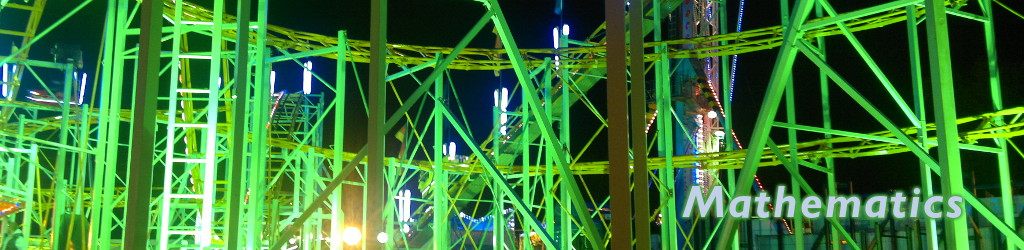
First we look at the regression parameters. The horizontal black line is zero and all regression parameters become close to the black line. This is exactly what we observed.

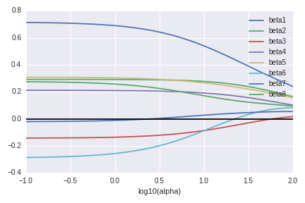
The next graph shows the eigenvalues of the covariance matrix of $\hat\beta(Y)$ (up to $\sigma^2$). These behave also as we expected.

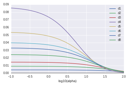
The third graph is the RMSE by $\lambda$. "alpha" in the image means $\lambda$. (This is the notion of scikit-learn.) When $\lambda \sim 1$, the predictive model seems trust (low variance) and accurate (low bias) at the same time.

Why we need to standardize the data

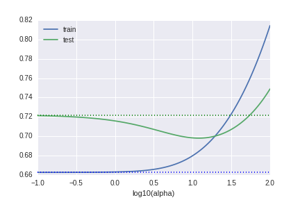
In our theoretical discussion we only need to centralise the data $X$ for our observation. But it could not enough to obtain a good result in practice. The ridge regression depends on the scale of the data. If we do not standardize the data, the graph of RMSE becomes as follows.

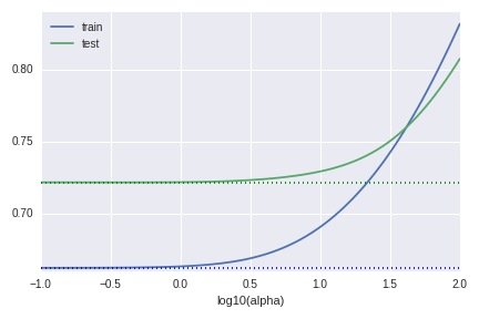
We can not improve the model at all.